Figure 1: Power/VSWR meter using ИН-13 neon bar-graph indicators. Click on the image for a larger version
In Part 1 I laid out the requirements of the ИН-13-based neon bar-graph VSWR/power meter. Admittedly, this is a "buy cool, old tech and figure out what project might use it" scenario - but having one tube always showing the forward power and the other tube showing either reverse power of calculated VSWR was the goal.
In the previous installment we talked about how to generate the high voltage (130 volts or so) for the bar-graph neons, the means to drive precise amounts of current through the tubes using precision current sink circuits, and the "Tandem" coupler to detect forward and reflected power.
Mounting the tubes
Figure 2: ИН-13 tubes in the raw. It is up to the constructor to determine how best to mount these tubes - and how to connect them to the circuit. Figure 3 shows how flexible wires were attached as the wires on the tubes themselves are very easily broken! Click on the image for a larger version.
In looking at Figure 1 you can see that the ИН-13 tubes are mounted to pieces of clear acrylic, but a quick look at Figure 2 shows that they don't really have a means of mounting, leaving the method to the imagination of the user.
In preparing the tubes for mounting I trimmed the wire leads and soldered flexible wires to them, covering them with "hot melt" (thermoset) adhesive to passivate the connection, making them relatively durable: The original wires will NOT tolerate much flexing at all and are likely to break off right at the glass "pinch" - which would make the tube useless. Figure 3 shows how the leads were encapsulated - the thermoset adhesive being tinted with a permanent marker - mainly to add a bit of color.
Laser-cut sheets and markings
Figure 3: Close-up of the "hot-glue" covered wire attachments for the ИН-13 tubes. Also visible are the black wire loops holding them in place and the laser-edged markings on the acrylic. Click on the image for a larger version.
In looking at Figure 1 and 3 you will also notice that there are scales indicating the function and showing scale graduations and the associated numerical values. I'm fortunate to have a friend (also an amateur radio operator) who has a high-power laser cutter and it was easy to lay out the precise dimensions of the acrylic sheets and also have it cut the holes for the mounting screws in the corners as well.
While it takes a bit of laser power to cut the sheets, a far lower power setting will ablate the surface, yielding a result not unlike surface engraving and when lit from the edges, these ablations will light up with the rest of the sheet remaining pretty dark: A total of four sheets were cut and "engraved" in this way: The front sheet for "VSWR" and its markings, the middle sheet for "Reverse Power" and the rear acrylic sheet for "Forward Power". It was possible to arrange the lettering so that only "VSWR" and "Reverse Power" were atop each other but in subdued light - and with a bit of darkened plastic in front of the display - the markings on the un-lit sheet are practically invisible. The fourth sheet mentioned was left blank, being the protective cover.
Edge lighting
Edge-lit displays go back decades - and the idea likely goes back centuries where it was observed that imperfections in glass (later, plastic) would be visible if the substrate was illuminated from the edge. Since the early-mid 20th century, one could find a number of edge-lit indicators - usually in some sort of test equipment of industrial displays - but they occasionally showed up in the consumer market - usually acrylic or similar with the markings engraved with a rotary tool or - as may be done nowadays, a laser.
While incandescent lamps would have been used in the past, LEDs are the obvious choice these days and for this I selected some "high brightness" LEDs to light the edges of the engraved acrylic sheets. For the "Forward Power" sheet - which would be that which was always illuminated in use - I chose white while using Green for VSWR and Blue for Reverse Power. I'd considered Yellow and Red, but discarded the former as it might appear too much light the white under some conditions and past experience has reminded me that - particularly in a dark room - the human eye can't see or focus on fine detail on red objects very easily.
Figure 4: Six LEDs are epoxied to the edge to evenly light the laser- etched markings in the acrylic sheet. The faces of the LEDs were filed flat to facilitate bonding and improve efficiency. Click on the image for a larger version.
Figure 4 shows some details as to how the edge lighting is accomplished. Six equally-spaced LEDs were epoxied to the bottom edge of the display, arranged to be nearly the width of the engraved text. In writing this entry I observed that photographing edge-lit displays such as this is nearly impossible owing to the variations in illumination (e.g. it's difficult to take pictures of very bright objects in the dark!) but the effect is very even as viewed by the human eye.
The six LEDs were connected as two series strings of three LEDs: As each LED requires about three volts - and I have only a 12 volt power source - doing so requires only a bit more than nine volts to power the LED arrays. As the green and white LEDs are also silicon nitride based as well, they take similar voltages.
Not readily apparent from Figure 4 is the fact that the LEDs were modified slightly. As we are trying to interface a standard T1-3/4 LED to the flat edge of a plastic sheet, it's apparent that the rounded, focused lens makes this physically difficult. To mitigate this, the top of the LED was flattened with a file and the clear epoxy was removed to just above the light emitting die. The result of this is that a flat surface is mated to another flat surface for a physically stronger bond and a more efficient coupling of light and a bit of the LED's original directivity in the form of the "lens" is removed from the equation.
Just prior to mounting the acrylic sheets in the "stack up" some black electrical tape was applied. This tape was put on both sides of the sheet, extending just above the bottom edge, to reduce the glare from the LEDs and to minimize the possibility of this light coupling into the adjacent sheet.
Mounting the tubes and sheets
As can be seen from Figure 3, the tubes are held in place with loop of solid-core insulated wire - the holes mounting them also "drilled" with the laser. The "stack-up" of acrylic sheets and the tubes - both of which were mounted on "VSWR" acrylic layer - is held together using 6-32 brass machine screws and spacers with a piece of 1/4" (5.2mm) plywood covered with black felt for the back to provide contrast.
The box and base
As can be seen from figure 1, the entire unit is in a wooden base: The same friend with the laser cutter also had some scraps of red oak and a simple base was made, decorated with an ogee cut around the perimeter with the router while atop it a simple box with mitered corners - facing at a slight upward angle - in which the display and electronics reside. On the base itself are two buttons: One switches between VSWR and Reverse Power and the other between peak and average readings. These switches have other functions as well, which will be discussed in the third installment when the final circuit and internal workings of the software is discussed.
Figure 1: Power/VSWR meter using ИН-13 (a.k.a. "IN-13") neon bar-graph indicators. Click on the image for a larger version.
Several years ago I bought some Soviet-era neon bar-graph displays - mainly because I thought that they looked cool, but I didn't have any
ideas for a specific project.
After mulling over possible uses for
these things for a year or so - trying to think of something other than
the usual audio VU meter or thermometer - I decided to construct a
visual watt/VSWR indicator for amateur radio HF use.
* * *
I actually bought two different types of these bar-graph tubes:
The ИН-9 (a.k.a. "IN-9"). This tube is 5.5" (140mm) long and 0.39" (10mm) diameter. It has two leads and the segments light up sequentially - starting from the end with the wires - as the current increases.
The ИН-13 (a.k.a "IN-13"). This neon bar-graph tube is about 6.3" (160mm) long and 0.39" (10mm) diameter. Like the ИН-9 its segments light up sequentially with increasing current but it has a third lead - the "auxiliary cathode" - that is tied to the negative supply lead via a 220k resistor that provides a "sustain" current to make it work more reliably at lower currents.
Note: It would be improper to refer to these as "Nixies" as that term refers to a specific type of numeric display - which these are not. Despite this, the term is often applied - likely for "marketing" purposes to get more hits on search engines.
Figure 2: A pair of ИН-13 neon indicator tubes. These tubes are slightly longer than than the ИН-9 tubes and have three leads Click on the image for a larger version.
For a device that is intended to indicate specific measurements, it's important that it is consistent, and for these neon indicators, that means that we want the bar graph to "deflect" the same amount anytime the same amount of current is applied to it. In perusing the specifications of both the ИН-9 and ИН-13 it appeared that the ИН-13 would be more suitable for our purposes.
This project would require two tubes:
Forward power indicator. This would always indicate the forward RF power as that was that's something that is useful to know at any time during transmitting.
Reverse power/VSWR.
This second tube would switchable between reverse power, using the same
scale as the forward power display, and VSWR - a measurement of the
ratio between forward and reverse power and a useful indicator of the
state of the match to the antenna/feedline.
Driving the tubes
"Because physics", gas discharge tubes require quite a bit of voltage to "strike" (e.g. light up) and these particular tubes need for their operation about 140 volts - a "modestly high" voltage at low current - only a few milliamps (less than 5) per tube, peak.
Figure 3:
Test circuit to determine the suitability of various inductors and transistors
and to determine reasonable drive frequencies. Diode "D" is a high-speed,
high-voltage diode, "R" can be two 10k 1 watt resistors in parallel and
"Q" is a power FET with suitably high voltage ratings (>=200 Volts)
and a gate turn-on threshold in the 2-3 volt range so that it is suitable
to be driven by 5 volt logic. V+ is from a DC power supply that is
variable from at least 5 volts to 10 volts. The square wave drive, from a
function generator, was set to output a 0-5 volt waveform to
make certain that the chosen FET could be properly driven by a 5 volt
logic-level signal from the PIC as evidenced by it not getting perceptibly
warm during operation.
The method used for this project and the aforementioned Zenith radio is boost-type converter as depicted in Figure 3.
The switching frequency must be pretty high - typically in the 5-30 kHz range if one
wishes to
keep the inductance and physical size of that inductor reasonably
small.
As in the case of the Zenith Transoceanic project, I used the PWM output of the microcontroller - a PIC - to drive the voltage converter with a frequency in the range of 20-50 kHz. For our needs - generating about 140 volts at, say, 15 milliamps maximum, I knew (from experience) that a 220uH choke would be appropriate. Figure 4, below, shows the as-built boost circuit.
Figure 4: The voltage boost converter section showing the transistor/inductor, rectification/filtering and voltage divider circuitry.
Description:
Q301 is a high-voltage (>=200 volt) N-channel MOSFET - this one being pulled from a junked PC power supply (the particular device isn't critical) which is driven by a square wave on the "HV_PWM" line from the microcontroller: R301, the 10k resistor, keeps the transistor in the "off" state when the controller isn't actively driving it (e.g. start-up). L301, a 220uH inductor, provides the conversion: When Q301 is on, the bottom end is shorted to ground causing a magnetic field to build up and when Q301 is turned off, this field collapses, dumping the resulting voltage through D301, which is a "fast" high voltage diode designed for switching supplies - a 1N4000 series diode would not be a good choice in this application as it's quite "slow".
R304, a 33k resistor, is used to provide a minimum load of the power supply, pulling about 4.25 mA at 140 volts: This "ballast" improves the ability of the supply to be regulated as the difference between "no load" (the neon bar-graphs energized, but with no "deflection") and full load (all segments of the tubes illuminated) is less than 4:1. The resistive divider of R302 and R303 is used to provide a sample of the output voltage to the microcontroller, yielding about 2.93 volts when the output is at 140 volts. The reader will, by now, likely have realized that I could have used R304 as part of the voltage divider - but since the value of this resistor was determined duringtesting, I didn't bother removing R302/R303 when I was done: Anyway, resistors are cheap!
Setting the current:
Having the 140 volt supply is only the first part of the challenge: As these tubes use current to set the "deflection" (e.g. number of segments) we need to be able to precisely set this parameter - independent of the voltage - to indicate a value with any reasonable accuracy. For this we'll use a "current sink".
Figure 5: The precision current sinks that drive the neon tubes precisely based on PWM-derived voltage. Click on the image for a larger version.
Figure 5, above, shows the driving circuits for the two tubes using the "precision current sink". Taking the top diagram as our example, we see that the inverting input of the op-amp (U401c) is connected to the junction of the emitter of Q401 and resistor R406. As is the wont of an op amp, the output will be driven high or low as needed to try to make the voltage (from the microcontroller) at pin 10 match that of pin 9 - in this case, based on feedback from the sense resistor, R406.
What this means is that as the transistor (Q401) is turned on, current will flow from the tube, through it and into R406 meaning that the voltage across R406 is proportional to the voltage on pin 10. It should be noted that current through R406 will include the current into the base - but this can be ignored as it will be only a tiny fraction (a few percent at most)of the total current. It's worth noting that this circuit is insensitive to the voltage - at least as long as such current can be sunk - making it ideal for driving a device like the ИН-13 (or ИН-9) in which its intended operation is dependent on the current rather than the operating voltage.
At this point it's worth noting that the driving voltages from the microcontroller ("FWD_PWM" and "REV_PWM") are not plain DC voltages, but rather from the 10 bit PWM outputs of the microcontroller. The use of a 10k resistor and 100nF (0.1uF) capacitors (R405 and C406, respectively) "smooth" the square-ish wave PWM into DC.
Q401 and Q402 were, again, random transistors that I found in scrapped power supplies, but since there's at least 70 volts drop across the tube, about any NPN transistor rated to withstand at least 80 volts should suffice. It's also worth noting the presence of R407, which provides the "sustain" current on the "auxiliary" cathode.
Figure 6: An exterior view of the tandem coupler module. Visible is the top shield and the three feedthrough capacitors used to pass voltage and block RF. Click on the image for a larger version.
RF sensing
For
sensing forward and reflected power I decided to use an external
"sensing head" that was connected inline with the radio, on the "tuner"
side of the feedline.
For sensing power in both directions I chose the
so-called "Tandem" coupler which consists of a through-line sampler in
which a short length of coaxial cable carrying the transmit power (T1 in the diagram of Figure 7) passes through a toroidal core -
using some of the original cable's braid grounded at just one end as a
Faraday shield. An identical transformer (T2) is connected across the first (T1) for symmetry.
When carefully
constructed this arrangement has quite good intrinsic directivity and a
wide frequency range. Figure 6 shows the diagram of this section.
Figure 7: Schematic diagram of the "Tadem" coupler. A bidirectional coupler sends power to separate AD8307 logarithmic amplifiers - one for forward and the other for reverse. The outputs, expressed in "volts/dB" are sent to the microcontroller. Click on the image for a larger version.
The
RF sensing outputs of the second tandem coupler (T2) then goes through resistive
voltage dividers (R606/R607 for the reverse sample and R603/604 for the forward sample) to a pair of Analog Devices AD8307 logarithmic
amplifiers - one for forward power and the other for reverse - to
provide a DC voltage that is logarithmically proportional to the
detected RF power. This voltage is then coupled through series resistors (for both RF and DC protection) R605/R608 and to the outside world using feedthrough capacitors.
The use of a logarithmic amplifier precludes the
need to have range switching on power meter as RF energy from well below
a watt to well over 2000 watts can be represented with only a few volts
swing. Looking carefully at Figure 6 one can see a label that notes that the response of the AD8307 is about 25 millivolts per dB - and this applies across the entire power range of a few hundred milliwatts to 2000 watts.
All
of this circuitry is mounted in a box constructed of circuit board
material and connected to the display unit with an umbilical cable that
conveys power and ground along with the voltages that indicates forward
and reflected power.
Figure 8: An inside view of the Tandem Match (sense unit) showing the coupling lines, internal shielding and AD8307 boards. Click on the image for a larger version.
Figure 8 shows the as-built "sense unit" and the two coaxial sense lines are clearly visible. As can be seen, the "main line" coupler is physically separated and shielded from the secondary sense line, using PTFE ("Teflon") feedthrough lines to pass the signals.
The AD8307 detectors themselves can be seen at the left and right edges of the lower half of the unit, built on small pieces of perfboard. All signals - including the 12 volt power and the DC voltages of the output pass through 4000pF feedthrough capacitors to prevent both ingress and egress of RF energy which could find its way into the '8307 detectors and skew readings.
* * * * *
In a future posting (Part 2) we'll talk about the final design and integration of this project.
The Chameleon SA-1 is a compact easy to use antenna analyzer that will help you measure SWR and tune your multi band antenna, like the Chameleon PRV System or Wolf River Coil Silver Bullet 1000. The meter measures SWR from 1:1 – 19.9 in a frequency range of 1.6 MHz to 160 MHz.
The Chameleon SA-1 is a compact lightweight SWR analyzer that would be perfect in your portable antenna kit. Opening the box you will find, a Nine volt battery, a BNC to UHF adapter, and the unit itself enclosed in a protective velvet bag.
The SA-1 has a continuous frequency range of 1.6 to 160 Mhz so it will be able to test the SWR for anyHF and VHF antennas in the amateur radio bands. It can also display the SWR from 1:1 up to 19.9:1 for that antenna. Run time with the battery is approximately 20 hours or 15 hours when you use the back light.
On the top of the meter is a small power switch, a BNC antenna port, and a socket that is labeled serial. We’ll talk about the serial feature in a bit. But first let’s look at the front of the unit
The SA-1 does not come with any instructions. Instead, everything you need to know to operate the meter is screen printed on the front of the unit. When you power on the meter, you will see the frequency and SWR on the dot matrix LCD display. Every time you turn on the unit, the frequency also defaults back to 14,000 Mhz. To adjust the frequency, you first tap the knob to select the digit and then rotate it to change the number. The unit is constantly testing the SWR, so there is nothing else you need to do. If you want to toggle the backlight, press and hold the center knob. That’s it. The SA-1 does one thing, and that’s measuring SWR. so there is nothing else you need to set it up.
A single function meter like this can be really handy in the field as it doesn’t distract with unnecessary features. It’s all in the goal of getting on the air quickly. So let’s see how fast we can do that as I demonstrate setting up and adjusting a multiband vertical antenna.
Timestamp 00:00:00 Chameleon SA-1 Antenna Analyzer 00:01:35 Features and Specs of the Chameleon SA-1 00:03:31 Using the SA-1 SWR Meter 00:13:15 Chameleon SA-1 Secret Feature 00:15:30 My thoughts on the SA-1 Antenna Analyzer
Links may be affiliate links. As an Amazon Associate, I earn from qualifying purchases. This does not affect the price you pay.
Last week, in response to a reader’s question here on QRPer.com, I was reminded that I hadn’t yet made a video specifically about my Mountain Topper MTR-3B SOTA field kit. Yesterday, I made a short video (see below) where I show what I pack in my MTR-3B field kit and why I choose to house … Continue reading Deep Dive: My Mountain Topper MTR-3B Watertight SOTA Field Kit→
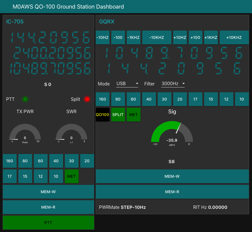
Following on from my article about my QO-100 Satellite Ground Station Complete Build, this article goes into some detail on the Node-RED section of the build and how I put together my QO-100 Satellite Ground Station Dashboard web app.
The Node-RED project has grown organically as I used the QO-100 satellite over time. Initially this started out as a simple project to synchronise the transmit and receive VFO’s so that the SDR receiver always tracked the IC-705 transmitter.
Over time I added more and more functionality until the QO-100 Ground Station Dashboard became the beast it is today.
M0AWS QO-100 Ground Station Control Dashboard built using Node-RED.
Looking at the dashboard web app it looks relatively simple in that it reflects a lot of the functionality that the two radio devices already have in their own rights however, bringing this together is actually more complicated than it first appears.
Starting at the beginning I use FLRig to connect to the IC-705. The connection can be via USB or LAN/Wifi, it makes no difference. Node-RED gains CAT control of the IC-705 via XMLRPC on port 12345 to FLRig.
To control the SDR receiver I use GQRX SDR software and connect to it using RIGCTL on GQRX port 7356 from Node-RED. These two methods of connectivity work well and enables full control of the two radios.
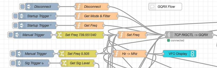
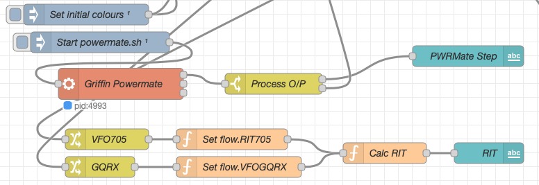
M0AWS Node-RED QO-100 Ground Station Dashboard Flow as of 12/06/24
The complete flow above looks rather daunting initially however, breaking it down into its constituent parts makes it much easier to understand.
There are two sections to the flow, the GQRX control which is the more complex of the two flows and the comparatively simple IC-705 section of the flow. These two flows could be broken down further into smaller flows and spread across multiple projects using inter-flow links however, I found it much easier from a debug point of view to have the entire flow in one Node-RED project.
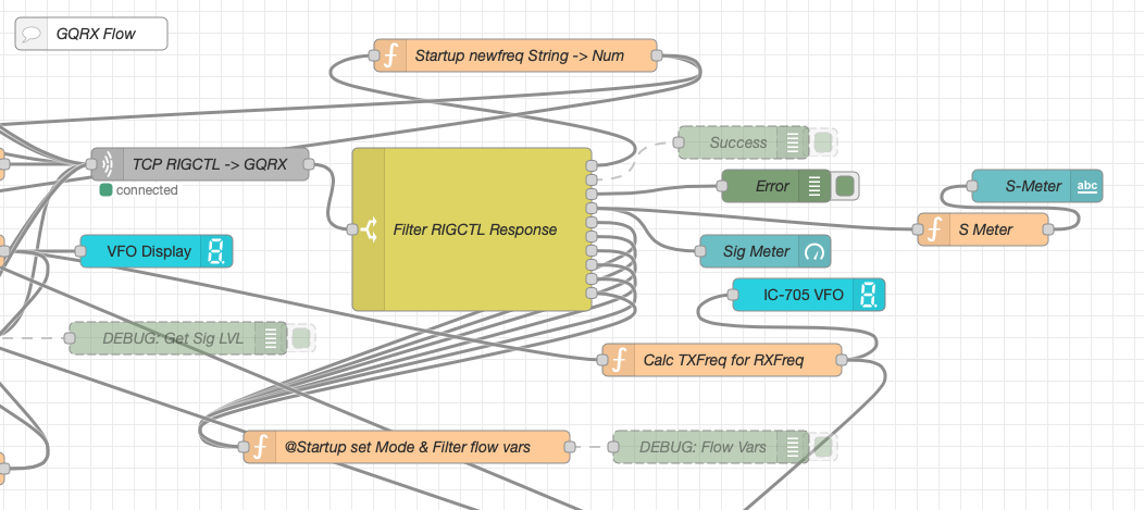
Breaking down the flow further the GQRX startup section (shown below) establishes communication with the GQRX SDR software via TCP/IP and gets the initial mode and filter settings from the SDR software. This information is then used to populate the dashboard web app.
M0AWS Node-RED QO-100 Ground Station Dashboard – GQRX Startup Flow
The startup triggers fire just once at initial startup of Node-RED so it’s important that the SDR device is plugged into the PC at boot time.
All the startup triggers feed information into the RIGCTL section of the GQRX flow. This section of the flow (shown below) passes all the commands onto the GQRX SDR software to control the SDR receiver.
M0AWS Node-RED QO-100 Ground Station Dashboard – GQRX RIGCTL Flow
The TCP RIGCTL -> GQRX node is a standard TCP Request node that is configured to talk to the GQRX software on the defined IP Address and Port as configured in the GQRX setup. The output from this node then goes into the Filter RIGCTL Response node that processes the corresponding reply from GQRX for each message sent to it. Errors are trapped in the green Debug node and can be used for debugging.
The receive S Meter is also driven from the the output of the Filter RIGCTL Response node and passed onto the S Meter function for formatting before being passed through to the actual gauge on the dashboard.
Continuing down the left hand side of the flow we move into the section where all the GQRX controls are defined.
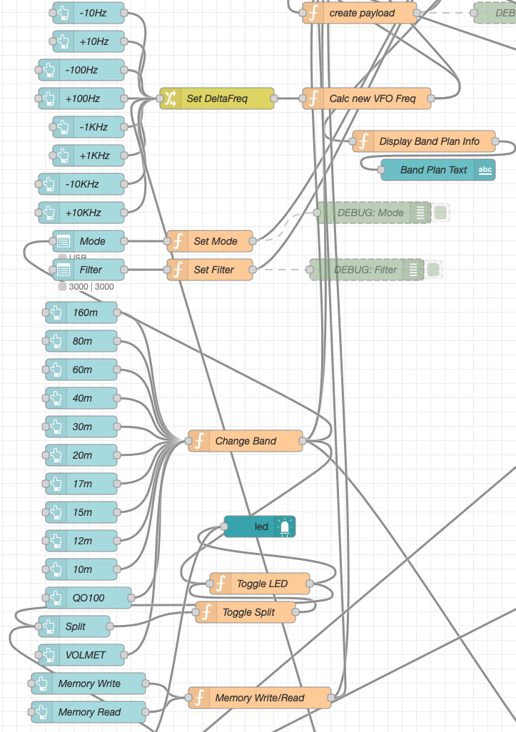
M0AWS Node-RED QO-100 Ground Station Dashboard – GQRX Controls Flow
In this section we have the VFO step buttons that move the VFO up/down in steps of 10Hz to 10Khz. Each button press generates a value that is passed onto the Set DeltaFreq change node and then on to the Calc new VFO Freq function. From here the new VFO frequency is stored and passed onto the communications channel to send the new VFO frequency to the GQRX software.
The Mode and Filter nodes are simple drop down menus with predefined values that are used to change the mode and receive filter width of the SDR receiver.
Below are the HAM band selector buttons, each of these will use a similar process as detailed above to change the VFO frequency to a preset value on each of the HAM HF Bands.
The QO-100 button puts the transmit and receive VFO’s into synchro-mode so that the receive VFO follows the transmit VFO. It also sets the correct frequency in the 739Mhz band for the downlink from the LNB in GQRX SDR software and sets the IC-705 to the correct frequency in the 2m VHF HAM band to drive the 2.4Ghz up-converter.
The Split button allows the receive VFO to be moved away from the transmit VFO for split operation when in QO-100 mode. This allows for the receive VFO to be moved away so that you can RIT into slightly off frequency stations or to work split when working DXpedition stations.
The bottom two Memory buttons allow you to store the current receive frequency into a memory for later recall.
At the top right of this section of the flow there is a Display Band Plan Info function, this displays the band plan information for the QO-100 satellite in a small display field on the Dashboard as you tune across the transponder. Currently it only displays information for the satellite, at some point in the future I will add the necessary code to display band plan information for the HF bands too.
The final section of the GQRX flow (shown below) sets the initial button colours and starts the Powermate USB VFO knob flow. I’ve already written a detailed article on how this works here but, for completeness it is triggered a few seconds after startup (to allow the USB device to be found) and then starts the BASH script that is used to communicate with the USB device. The output of this is processed and passed back into the VFO control part of the flow so that the receive VFO can be manually altered when in split mode or in non-QO-100 mode.
M0AWS Node-RED QO-100 Ground Station Dashboard – Powermate VFO Flow
The bottom flows in the image above set some flow variables that are used throughout the flow and then calculates and sets the RIT value on the dashboard display.
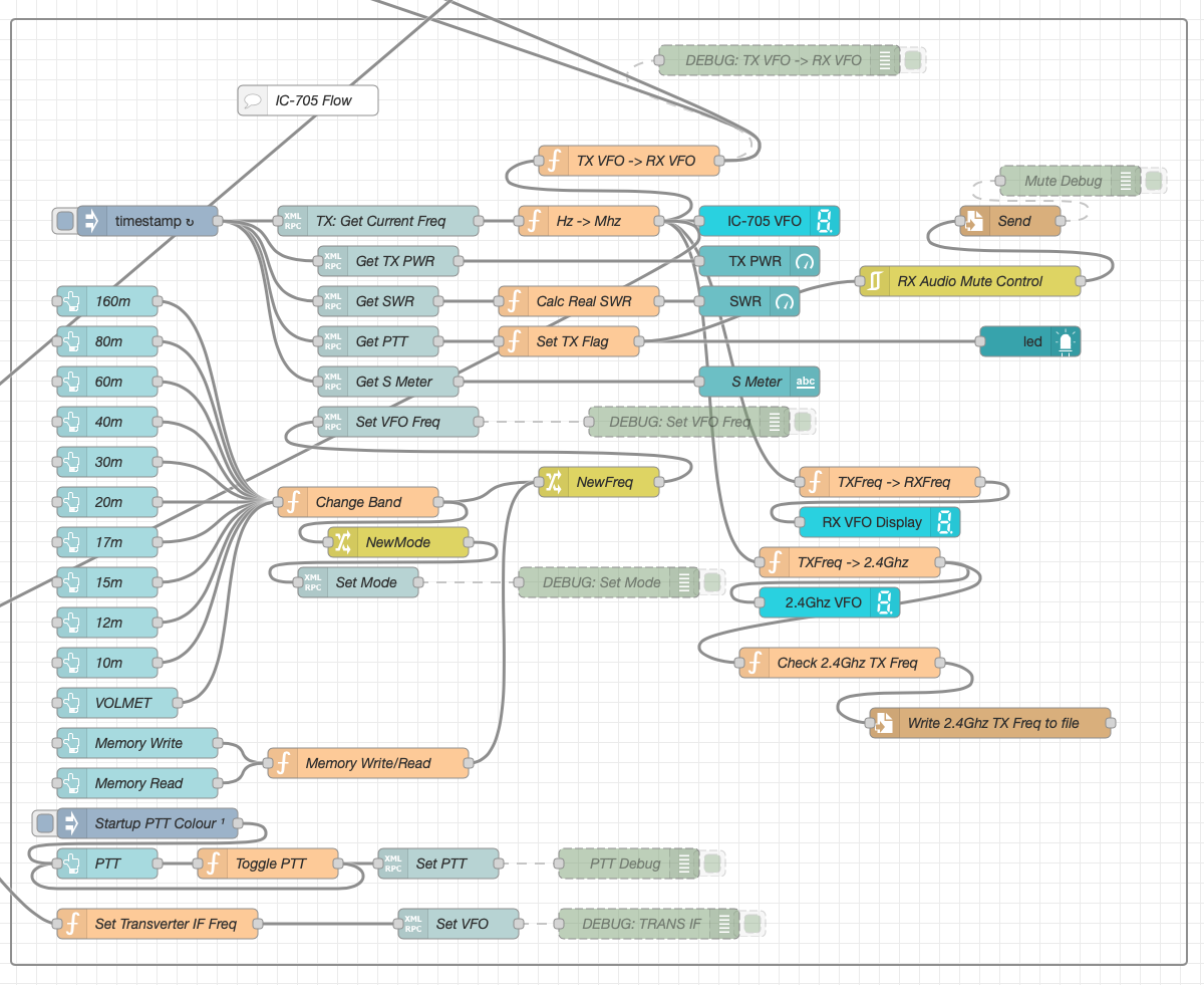
The final section of the flow is the IC-705 control flow. This is a relatively simple flow that is used to both send and receive data to/from the IC-705, process it and pass it on to the other parts of the flow as required.
M0AWS Node-RED QO-100 Ground Station Dashboard – IC-705 Control Flow
The IC-705 flow is started via the timestamp trigger at the top left. This node is nothing more than a trigger that fires every 0.5 seconds so that the dashboard display is updated in near realtime. The flow is pretty self explanatory, in that it collects the current frequency, transmit power, SWR reading, PTT on/off status and S Meter reading each time it is triggered. This information is then processed and used to keep the dashboard display up to date and to provide VFO tracking information to the GQRX receive flow.
On the left are the buttons to change band on the IC-705 along with a button to tune to the VOLEMT on the 60m band. Once again there two memory buttons to save and recall the IC-705 VFO frequency.
The Startup PTT Colour trigger node sets the PTT button to green on startup. The PTT button changes to red during transmit and is controlled via the Toggle PTT function.
At the very bottom of the flow is the set transverter IF Freq function, this sets the IC-705 to a preselected frequency in the 2m HAM band when the dashboard is switched into QO-100 mode by pressing the QO-100 button.
On the right of the flow there is a standard file write node that writes the 2.4Ghz QO-100 uplink frequency each time it changes into a file that is used by my own logging software to add the uplink frequency into my log entries automatically. (Yes I wrote my own logging software!)
The RX Audio Mute Control filter node is used to reduce the receive volume during transmit when in QO-100 full duplex mode otherwise, the operator can get tongue tied hearing their own voice 250ms after they’ve spoken coming back from the satellite. This uses the pulse audio system found on the Linux platform. The audio is reduced to a level whereby it makes it much easier to talk but, you can still hear enough of your audio to ensure that you have a good, clean signal on the satellite.
As I said at the beginning of this article, this flow has grown organically over the last 12 months and has been a fun project to put together. I’ve had many people ask me how I have created the dashboard and whether they could do the same for their ground station. The simple answer is yes, you can use this flow with any kind of radio as long as it has the ability to be controlled via CAT/USB or TCP/IP using XMLRPC or RIGCTL.
To this end I include below an export of the complete flow that can be imported into your own Node-RED flow editor. You may need to make changes to it for it to work with your radio/SDR but, it shouldn’t take too much to complete. If like me you are using an IC-705 and any kind of SDR controlled by GQRX SDR software then it’s ready to go without any changes at all.
In my quest to improve my Meshtastic signal range using home-brew antennas I’ve finally put together a neat little ground plane vertical antenna for the 868Mhz ISM band.
The design follows the normal ground plane simplicity using 4 radials and a vertical radiating element albeit on a tiny scale. The radiating element is 82mm long and the radials are each 92mm long.
M0AWS 868Mhz Ground Plane Vertical Antenna
Initially I modelled the antenna at a height of 3m above the ground with the radials tilted downwards at 45 degrees. I took this approach as this is how I have built ground plane verticals for the 70cm band in the past and so I thought I’d try the same approach on the 868Mhz ISM band. (I later found this to be detrimental to tuning!)
The 3D far field plot for the antenna shows it has a very nice, relatively high gain lobe at just 2 degrees elevation with a number of lower gain lobes higher up.
M0AWS 868Mhz Ground Plane Vertical Antenna 3D Far Field Plot
Looking at the 2D far field plot you can get a better understanding of the radiation pattern and gain figures at various angles. At 2 degrees there is 6.7dBi gain with the next major lobe being at 8 degrees with 4.36dBi gain, far more than I imagined I’d see for such a simple antenna.
M0AWS 868Mhz Ground Plane Vertical Antenna 2D Far Field Plot
Putting the antenna together was easy enough with particular attention being paid to the measurements of both the radials and radiating element. I soldered some lugs to the ends of the 2.5mm diameter solid core wire radials to enable easy attachment to the N Type chassis socket that I decided to use as the base for the antenna. This worked out well and provided a good solid mechanical and electrical connection for the 4 radials.
For the radiating element I used an N Type plug with the vertical 2.5mm solid core wire element soldered to the inner centre pin of the male connector. I also slid a small piece of insulation down the wire to stop it from shorting against the metal outer of the plug and then pushed in a tight rubber plug to stop water ingress.
M0AWS 868Mhz Ground Plane Antenna Close Up
Connecting my VNA I found the antenna was mostly resonant at 790Mhz with an SWR of 2.5:1. I knew this would be the case and that the wires would need a little trimming.
Trimming the wires a couple of times in 1mm nibbles I got the point of resonance up to 868Mhz but, the antenna was still exhibiting a lot of reactance that was keeping the SWR above 2:1. Trimming the radials reduced this slightly but, I could not get an SWR much lower than 1.95:1.
Scratching my head I decided to try moving the radials back up so that they were horizontal rather than at 45 degrees downwards, this had the immediate effect of the SWR dropping to 1.1:1.
M0AWS A rather fuzzy photo of the 868Mhz SWR curve for the GP Antenna
The SWR stays below 1.2:1 from 868Mhz to 871Mhz which is plenty wide enough for the Meshtastic devices. Why there is so much reactance when the radials are bent down at 45 degrees I am not sure, but it was easy enough to resolve.
M0AWS 868Mhz Ground Plane Antenna
The finished antenna is tiny but, seems to work well. Signals from my other nodes are up by 6-9dB according to the SNR reports in the Meshtastic app. I now need to make a couple more of these for my other nodes and then hope to hear some other nodes locally once they appear on air.
Remodelling the antenna in EzNEC with the radials as shown above the gain at 2 degrees is now 5.5dBi, down 1.2dBi but, the overall radiation pattern is identical to the original.
Total cost of the build is about £1 and an hour of my time tinkering with it, bargain!
Following on from my last article on improving the Heltec ESP32 v3 antennas I found during the installation of the 90 degree SMA connector that the device was very sensitive to stray capacitance from things around it. After reconnecting my VNA I found the SWR curve would change substantially depending on what the device was near and so I set about rectifying this.
I decided to remove all the insulation from the single radial inside the unit and then added two more radials to increase the ground for the antenna to tune against. I then removed the N type plug with the antenna connected to it and made a new antenna from a piece of 1.5mm solid core insulated mains wire connected directly to the N type socket, without using an N type plug. Tuning to resonance was much easier than before and I soon had the SWR down to 1.2:1. Moving the device around and placing near to other objects the SWR curve was now much more stable than before with only very slight changes in curve shape.
M0AWS Updated 868Mhz Antenna
Making this change to the 868Mhz antenna has shown an improvement in signal strength from my node-1 device of almost +0.5dB, every dB counts when you only have 100mW to play with!
The Bluetooth antenna update has made a massive improvement to the usability of the device via the iOS Meshtastic app. Being able to have a reliable, solid connection from anywhere in the house is great and I no longer lose messages because I’ve strayed outside the range of the Bluetooth connection.
I now have 2 new Heltec ESP32 v3 devices on the way to me and will be getting those configured and operational outside with external antennas in the hope of hearing some nodes locally to me.
I’ve been doing some antenna modelling and comparisons for John, W2VP comparing some phased and parasitic arrays. One of the phased arrays I modelled was an End-Fed-Half-Wave (EFHW) phased vertical array for the 40m band. It’s got such a nice radiation pattern that I thought I’d add it to my antenna pages here on the website for others to read too.
M0AWS 40m Band EFHW Phased Vertical Array Antenna View
The EFHW Vertical Phased Array is as simple as two vertical half wave wires both of which are fed via their own 49:1 Unun. Wire 1 (radiator) is exactly 20m tall and wire 2 (reflector) is 21m tall. The space between them is exactly 10.5m.
This simple antenna arrangement gives a surprisingly good radiation pattern with a reasonable forward gain and front-to-back (FB) ratio.
M0AWS 40m Band EFHW Phased Vertical Array 3D Far Field Plot
The antenna has quite a wide beam width which is to be expected from a pair of phased verticals. The nice thing about this array is that it has very little in the way of high angle radiation. This makes this antenna ideal for long distance communications. This isn’t an antenna for local chatter!
M0AWS 40m Band EFHW Phased Vertical Array 2D Far Field Plot
The 2D Far Field Plot shows that the antenna has a forward gain of 3.16dBi at 19 degrees. This is some 8 degrees lower than a typical 1/4 wave vertical phased array. The array also has a very respectable front-to-back (FB) ratio of 20.53dB.
Both elements in the array will need to be fed via individual 49:1 Ununs with the reflector requiring a feed phase angle of 100 degrees. A 100 degree phase angle gives better performance than the typical 90 degree phase angle that is typically used for 1/4 wave arrays.
For such a simple design this antenna should give great DX results as long as you have the necessary supports for the two vertical wires and the space for the guy lines. If only my garden was much bigger and I had some large trees to hand!
Summary:
Radiator (Element 1): 20m Reflector (Element 2): 21m Reflector Feed Phase Angle: 100 Deg Wire Dia: 4mm Feed Type: 49:1 Unun on each vertical element and a phasing harness Impedance: 50 Ohm SWR: <1.5:1 across whole band
I recently put up a 38m Inverted-L antenna (10m vertical/28m horizontal) and tuned it on the 160m band using a home-brew Pi-Network ATU. It’s working great on top band and I’m really pleased with performance so far.
I decided today that it would be good to try the inverted-L out on some of the other low bands too. Since my other HF antenna is a large vertical that’s great for DXing but, terrible for Inter-G I thought perhaps the Inverted-L would fill the inter-G gap.
M0AWS Pi-Network ATU using my JNCRadio VNA to find the ATU setting for each band
Having recently purchased a JNCRadio VNA from Martin Lynch and Sons it made tuning the ATU for each band really easy. When it comes to antenna resonance I like my antennas to have an SWR of less than 1.2:1. With the VNA connected it is really easy to tune the antenna for a 1:1 SWR on a particular frequency, make a note of the tune information and then move to the next frequency and start again.
M0AWS Pi-Network ATU Inductor with turns countM0AWS Pi-Network ATU Capacitor 1 and 2 settings
I marked up each turn on the large copper inductor so I could record the position of the input wire onto the inductor. I then added some markings on the two capacitors of the Pi-Network ATU for the resonance points on each band/frequency I wanted to resonate the antenna on.
M0AWS Pi-Network ATU settings noted for each band
After about 40mins I had all the settings recorded on a pad ready for testing from the shack end of the coax run. Connecting my Yaesu FTDX10 to the coax I ran through each band setting checking the SWR as I went. All bands tuned up perfectly 160m through 30m and receiving of Inter-G on the bands that were active was excellent.
Wanting to test the antenna on 40m for the first time I found Nick, M7NHC calling CQ and gave him a call using just 5w output. He came straight back to me and we had a quick chat.
Nick was using an Icom IC-7300 using just 10w into an end-fed long wire from Eastbourne down on the south coast so, we were both QRP. Nick was a 5/7 with QSB and he gave me a 5/8 with QSB, not bad at all consider how much power we were using.
I’m hoping to have a chat with some of the guys from the Matrix this evening on 60m SSB so, it will be interesting to see how the antenna performs on 5Mhz.
Since setting up the new HAM station here in the UK the one band I’ve not yet got back onto is 160m, one of my most favourite bands in the HF spectrum and one that I was addicted to when I live in France (F5VKM).
Having such a small garden here in the UK there is no way I can get any type of guyed vertical for 160m erected and so I needed to come up with some sort of compromise antenna for the band.
Only being interested in the FT4/8 and CW sections of the 160m band I calculated that I could get an inverted-L antenna up that would be reasonably close to resonant. It would require some additional inductance to get the electrical length required and some impedance matching to provide a 50 Ohm impedance to the transceiver.
Measuring the garden I found I could get a 28m horizontal section in place and a 10m vertical section using one of my 10m spiderpoles. This would give me a total of 38m of wire that would get me fairly close to the quarter wave length.
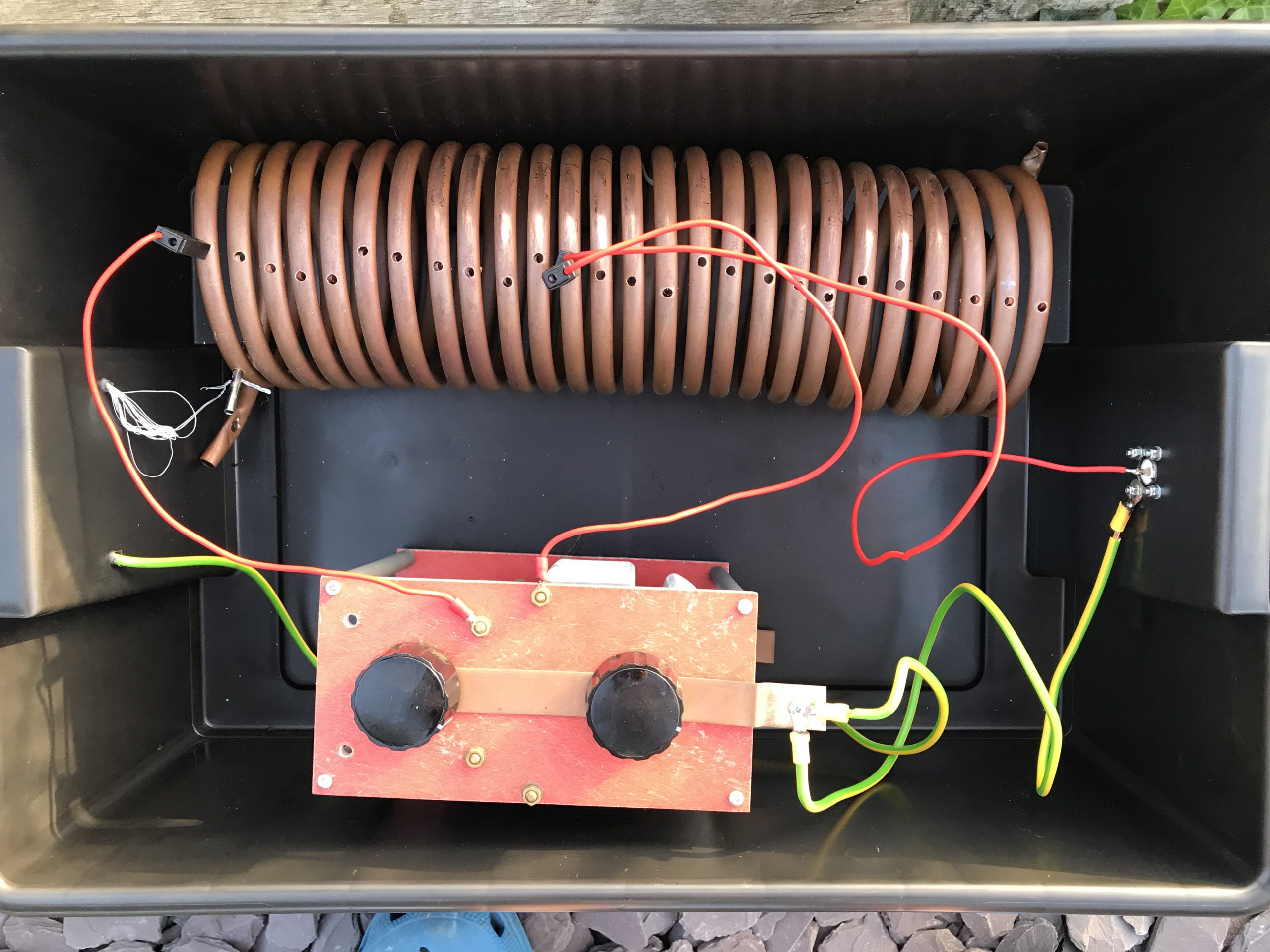
For impedance matching I decided to make a Pi-Network ATU. I’ve made these in the past and found them to be excellent at matching a very wide range of impedances to 50 Ohm.
M0AWS Homebrew Pi-Network ATU
Since I still had the components of the Pi-Network ATU that I built when I lived in France I decided to reuse them as it saved a lot of work. The inductor was made from some copper tubing I had left over after doing all the plumbing in the house in France and so it got repurposed and formed into a very large inductor. The 2 x capacitors I also built many years ago and fortunately I’d kept locked away as they are very expensive to purchase today and a lot of work to make.
Getting the Inverted-L antenna up was easy enough and I soon had it connected to the Pi-Network ATU. I ran a few radials out around the garden to give it something to tune against and wound a 1:1 choke balun at the end of the coax run to stop any common mode currents that may have appeared on the coax braid.
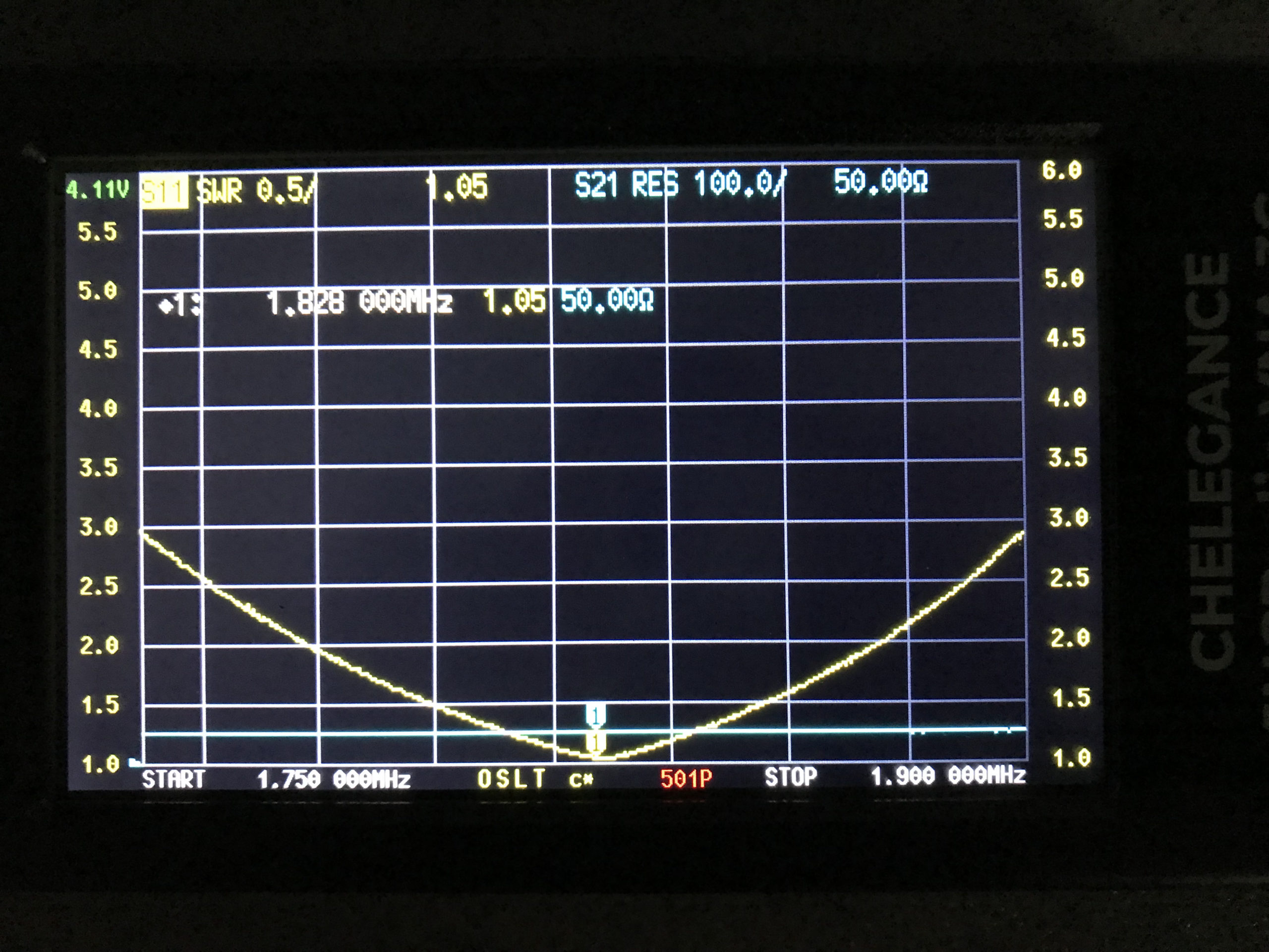
Connecting my JNCRadio VNA I found that the Inverted-L was naturally resonant at 2.53Mhz, not too far off the 1.84Mhz that I needed. Adding a little extra inductance and capacitance via the ATU I soon had the antenna resonant where I wanted it at the bottom of the 160m band.
M0AWS 160m Inverted L Antenna SWR Curve
With the SWR being <1.5:1 across the CW and FT8 section of the band I was ready to get on 160m for the first time in a long.
Since it’s still summer in the UK I wasn’t expecting to find the band in very good shape but, was pleasantly surprised. Switching the radio on before full sunset I was hearing stations all around Europe with ease. In no time at all I was working stations and getting good reports using just 22w of FT8. FT8 is such a good mode for testing new antennas.
As the sky got darker the distance achieved got greater and over time I was able to work into Russia with the longest distance recorded being 2445 Miles, R9LE in Tyumen Asiatic Russia.
In no time at all I’d worked 32 stations taking my total 160m QSOs from 16 to 48. I can’t wait for the long, dark winter nights to see how well this antenna really performs.
M0AWS Map showing stations worked on 160m using Inverted L Antenna
The map above shows the locations of the stations worked on the first evening using the 160m Inverted-L antenna. As the year moves on and we slowly progress into winter it will be fun to start chasing the DX again on the 160m band..
UPDATE 6th October 2023. Been using the antenna for some time now with over 100 contacts on 160m. Best 160m DX so far is RV0AR in Sosnovoborsk Asiatic Russia, 3453 Miles using just 22w. Pretty impressive for such a low antenna on Top Band.
This is a 15m band delta loop design that I’ve put together as requested by Wim, PE1PME.
The 15m band delta loop follows exactly the same design principles as all the other delta loop designs I’ve already put on the website. They are designed such that they present a 50 ohm impedance at the feed point and thus have no requirement for complex impedance matching circuits/transformers.
15m Band Delta Loop Antenna View
The dimensions for the antenna are as follows:
Wire 1 – Horizontal exactly 1m above the ground for its entire 7m length. Wires 2 & 3 are exactly 4.12m long each with the top being 3.18m above the ground.
15m Band Delta Loop Antenna 3D Far Field Plot
The 3D far field plot shows a typical delta loop radiation pattern with the maximum radiation through the loop and a deep null in the centre.
15m Band Delta Loop Antenna 2D Far Field Plot
The 2D elevation plot shows that the antenna will give a maximum gain of 1.5dBi at 26 degrees with useful gain at lower angles.
The SWR plot shows that the antenna will have a fairly wide bandwidth and match to 50 ohm coax extremely well. The antenna is designed to be fed in one of the lower corners via a 1:1 balun for best results.
15m Band Delta Loop Antenna SWR Curve
Summary:
Total Wire Length: 15.24m Horizontal Wire Length: 7m @ 1m above ground Diagonal Wire Lengths: 4.12m Wire Dia: 2.5mm Height at Centre: 3.18m Feed Type: 1:1 Balun in bottom corner (Can use coax if necessary) Impedance: 50 Ohm SWR: <1.5:1 at resonance
Since purchasing my Retevis RT85 2m/70cm handheld radio I’ve noticed that it seems rather deaf when using the antenna that came with the radio and isn’t as strong into the local repeaters as I imagined it would be.
Considering the local 2m and 70cm repeater isn’t that far from my QTH and there is pretty much a clear line of site view in the direction of the repeater I was somewhat surprised that on 70cm the repeater never breaks the squelch, even if it is set on it’s lowest setting of zero.
M0AWS Retevis RT85 dual band VHF/UHF Handheld Radio
Connecting my home made end fed dual band vertical dipole at 10m above ground the performance of the radio improves drastically as one would expect.
Having recently purchased a JNCRadio VNA 3G antenna analyser I decided to connect the Retevis supplied antenna to the analyser and see what the resonance was like on the two bands.
The antenna is labelled as 136-174Mhz and 400-470Mhz. This is an extremely wide frequency range for such a small antenna and clearly isn’t going to perform that well over such a wide bandwidth.
Connecting the antenna to the VNA and setting the stimulus frequency range to 144-148Mhz I found that the SWR curve of the antenna wasn’t particularly good.
M0AWS Retevis RT85 Antenna SWR Curve 2m
As shown above the SWR curve on the 2m Band is pretty poor. At 144.0Mhz it’s just over 3:1, at 145.496 (closest I could get to the 145.500 calling channel) the SWR is still 2.1:1. The antenna doesn’t really get close to resonance until 148Mhz where the SWR is 1.46:1.
With an SWR this high the radio will almost certainly be reducing the O/P power considerably to protect the PA stage from over heating due to so much power be reflected back into the transmitter. This explains the poor performance when using 2m repeaters locally and the somewhat limited range when using the OEM supplied antenna.
Looking at the SWR curve on the 70cm band, the antenna is much closer to resonance than it is on the 2m band but, it’s still not perfect.
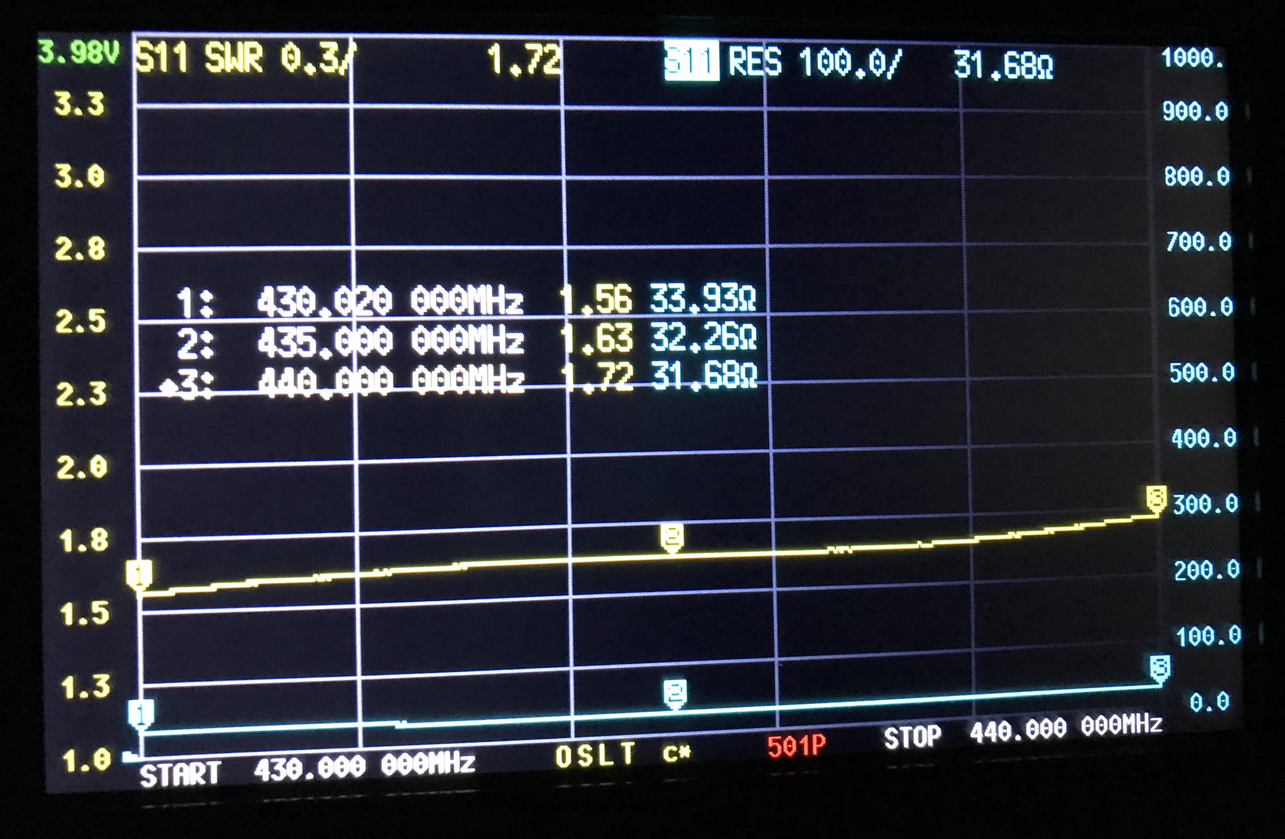
M0AWS Retevis RT85 Antenna SWR Curve 70cm
At 430Mhz the SWR is 1.56:1, at 435Mhz 1.63:1 and 440Mhz 1.72:1. Since the antenna is much closer to resonance on the 70cm band I would expect it to perform better than it does.
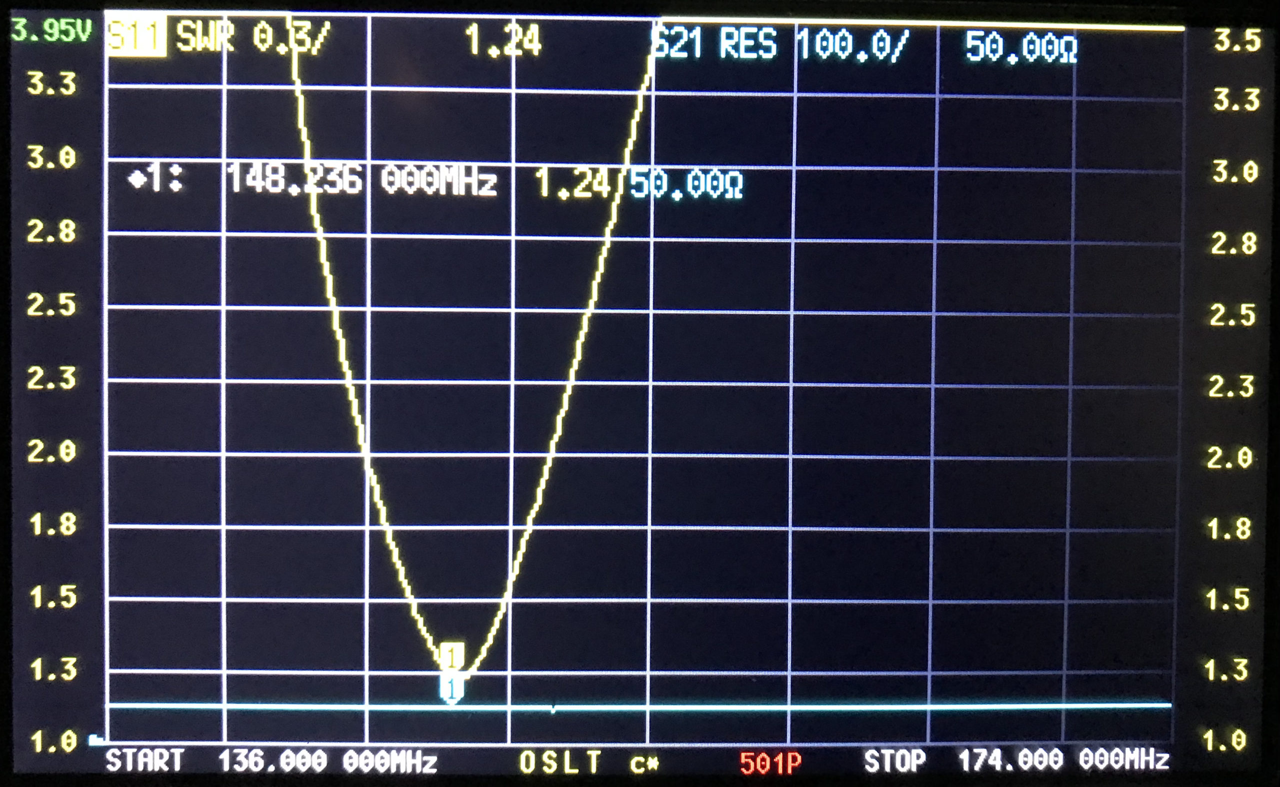
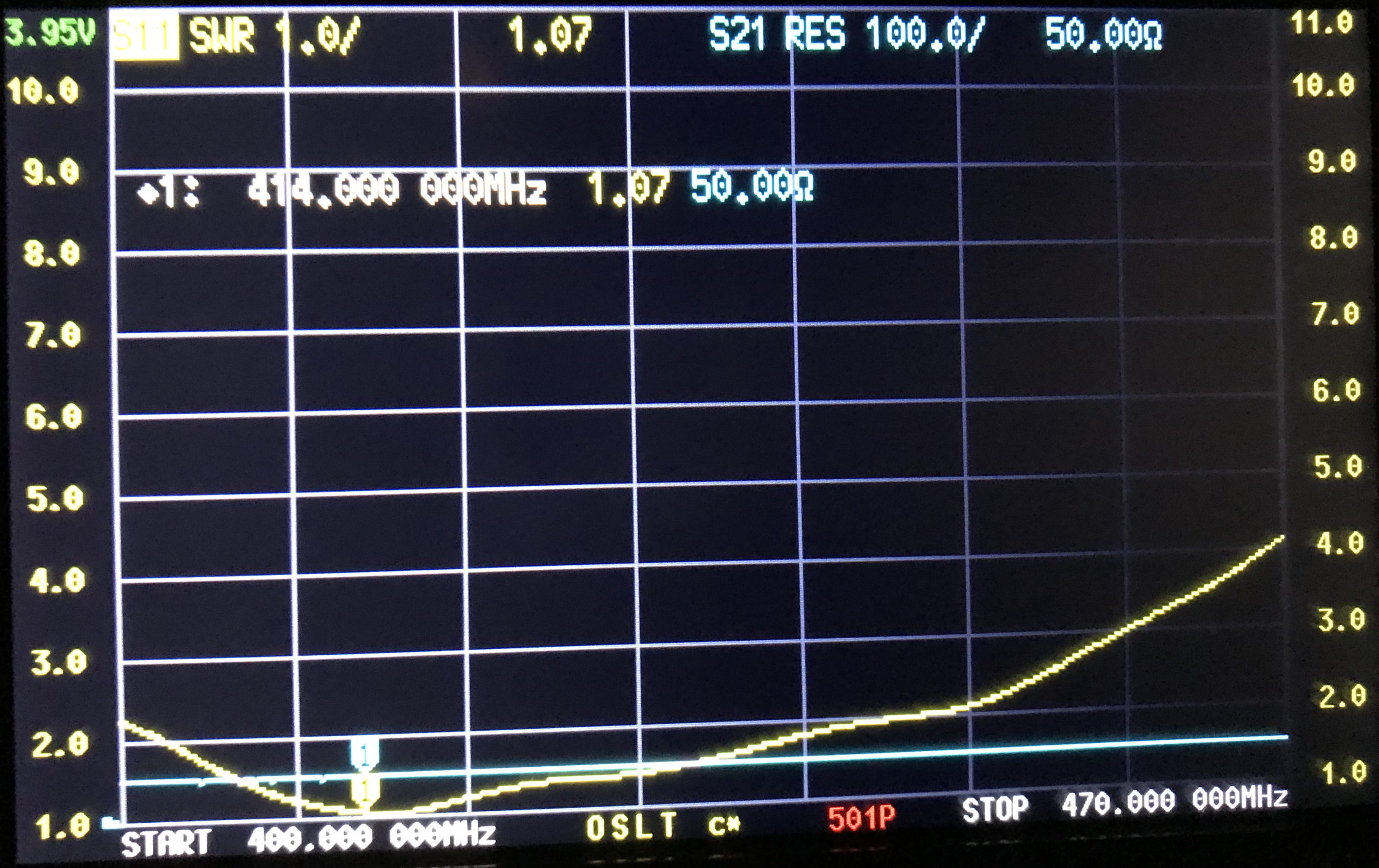
Looking at the SWR curves over the entire supported frequency range of 136-174Mhz and 400-470Mhz, there is only one point of resonance on VHF around 148Mhz and on UHF around 400Mhz.
With such disappointing performance on both VHF and UHF I’ve decided to investigate making my own 2m/70cm antenna for the handheld to see if I can improve both the SWR on each band and the overall performance of the radio.
Many years ago I had an MFJ-259B antenna analyser that I used for all my HF antenna projects. It was a simple device with a couple of knobs, an LCD display and a meter but, it provided a great insight into the resonance of an antenna.
MFJ-259B Antenna Analyser
Today things have progressed somewhat and we now live in a world of Vector Network Analysers that not only display SWR but, can display a whole host of other information too.
Being an avid antenna builder I’ve wanted to buy an antenna analyser for some time but, now that I’m into the world of QO-100 satellite operations using frequencies at the dizzy heights of 2.4GHz I needed something more modern.
If you search online there are a multitude of Vector Network Analysers (VNAs) available from around the £50.00 mark right up to £1500 or more. Many of the VNAs you see on the likes of Amazon and Ebay come out of China and reading the reviews they aren’t particularly reliable or accurate.
After much research I settled on the JNCRadio VNA 3G, it gets really good reviews and is very sensibly priced. Putting a call into Gary at Martin Lynch and Sons (MLANDS) we had a long chat about various VNAs, the pros and cons of each model and the pricing structure. It was tempting to spend much more on a far more capable device however, my sensible head kicked in and decided many of the additional features on the more expensive models would never get used and so I went back to my original choice.
Gary and I also had a long chat about building a QO-100 ground station, using NodeRed to control it and how to align the dish antenna. The guys at MLANDS will soon have a satellite ground station on air and I look forward to talking to them on the QO-100 transponder.
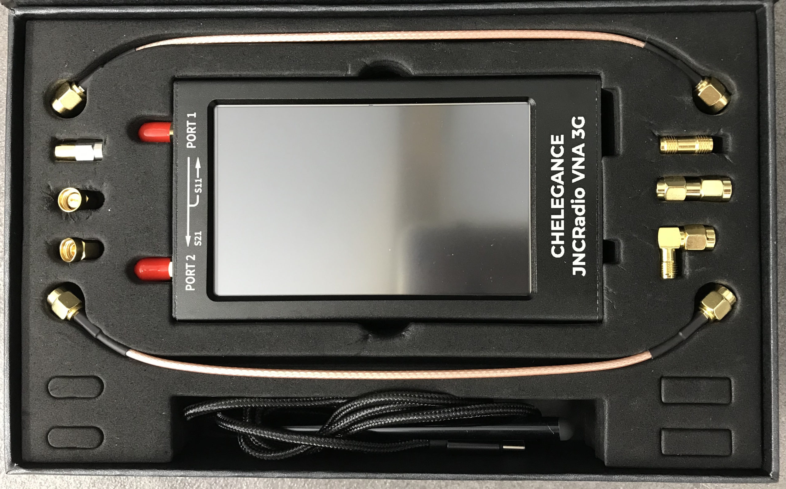
M0AWS – JNCRadio VNA 3G PackagingM0AWS – JNCRadio VNA 3G in box with connectors and cables
Initially I wanted to check the SWR of my QO-100 2.4GHz IceCone Helix antenna on my satellite ground station to ensure it was resonant at the right frequency. Hooking the VNA up to the antenna feed was simple enough using one of the cables provided with the unit and I set about configuring the start and stop stimulus frequencies (2.4GHz to 2.450GHz) for the sweep to plot the curve.
The resulting SWR curve showed that the antenna was indeed resonant at 2.4GHz with an SWR of 1.16:1. The only issue I had was that in the bright sunshine it was hard to see the display and impossible to get a photo. Setting the screen on the brightest setting didn’t improve things much either so this is something to keep in mind if you plan on using the device outside in sunny climates.
(My understanding is that the Rig Expert AA-3000 Zoom is much easier to see outside on a sunny day however, it will cost you almost £1200 for the privilege.)
A couple of days later I decided to check the SWR of my 20m band EFHW vertical antenna. I’ve known for some time that this antenna has a point of resonance below 14MHz but, the SWR was still low enough at the bottom of the 20m band to make it useable.
Hooking up the VNA I could see immediately that the point of resonance was at 13.650Mhz, well low of the 20m band and so I set about shortening the wire until the point of resonance moved up into the band.
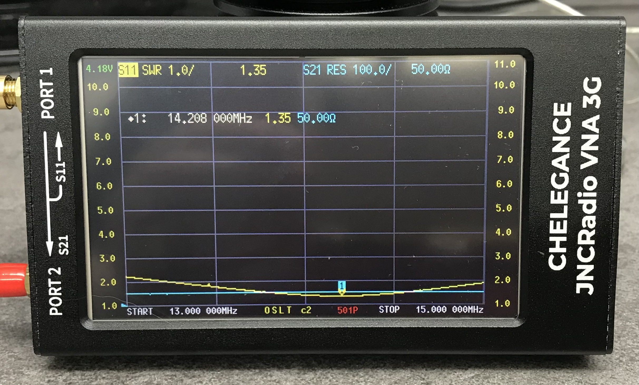
JNCRadio VNA3G showing 20m Band EFHW Resonance
With a little folding back of wire I soon had the point of resonance nicely into the 20m band with a 1.35:1 SWR at 14.208Mhz. This provides a very useable SWR across the whole band but, I decided I’d prefer the point of resonance to be slightly lower as I tend to use the antenna mainly on the CW & FT4/8 part of the band with my Icom IC-705 QRP rig.
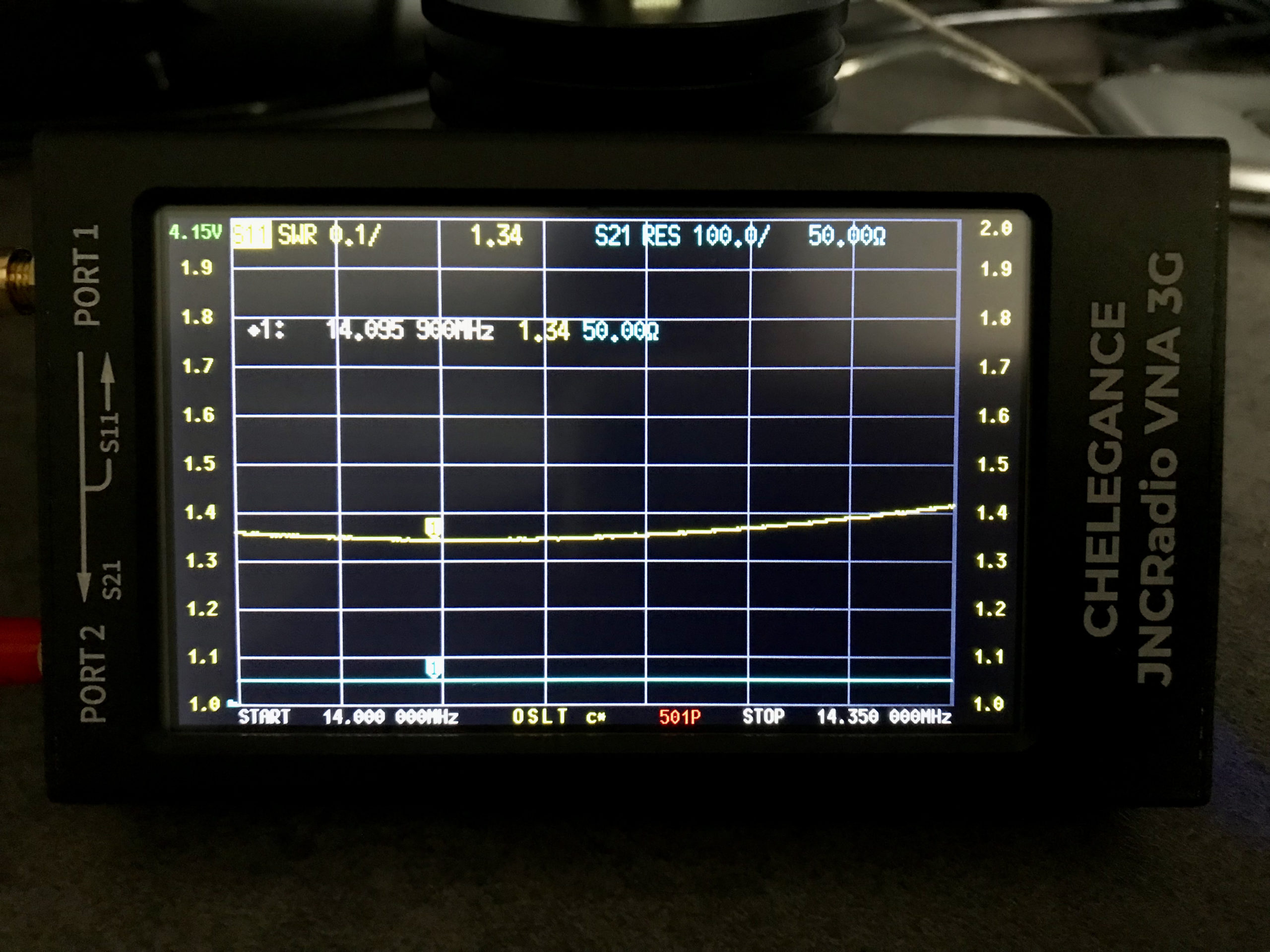
Popping out into the garden once more I lengthened the wire easily enough by reducing the fold back and brought the point of resonance down to 14.095Mhz.
JNCRadio VNA3G showing 20m Band EFHW Resonance 14Mhz to 14.35Mhz Sweep
The VNA automatically updated the display realtime to show the new point of resonance on the 4.3in colour screen. I also altered the granularity of the SWR reading on the Y axis to show a more detailed view of the curve and reduced the frequency range on the X axis so that it showed a 14Mhz to 14.35Mhz sweep. With an SWR of 1.34:1 at 14.095Mhz and a 50 Ohm impedance, the antenna is perfectly resonant where I want it.
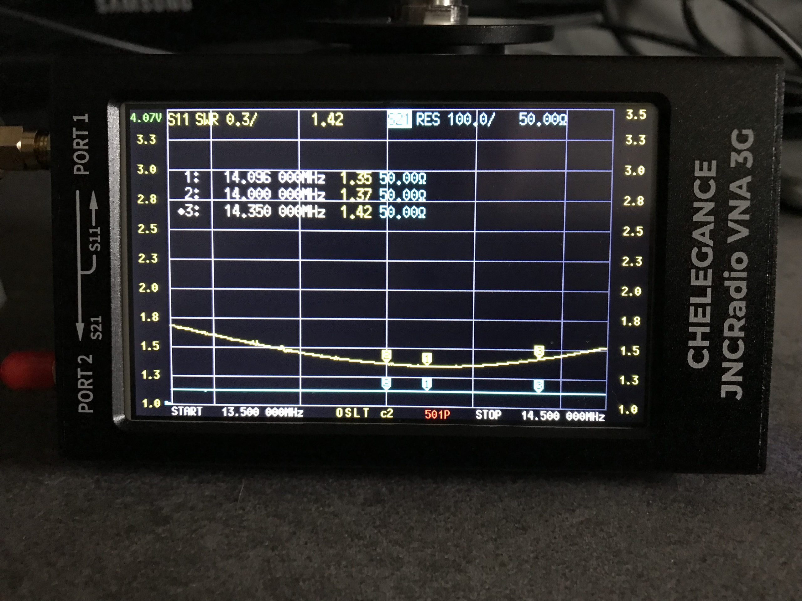
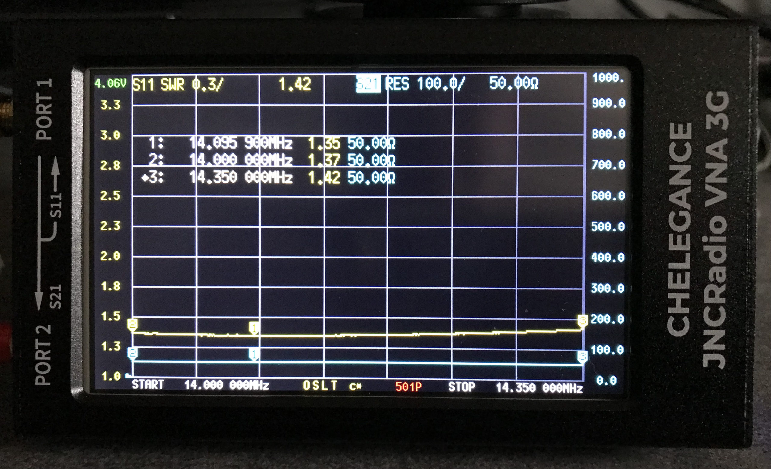
It’s interesting to note that the antenna is actually useable between 13.5Mhz and 14.5Mhz with a reasonable SWR across the entire frequency spread. Setting 3 markers on the SWR curve I could see at a glance the SWR reading at 14Mhz (Marker 2) , 14.350Mhz (Marker 3) and the minimum SWR reading at 14.095Mhz (Marker 1).
Last year, I was "car camping" with a bunch of friends - all of which happened to be amateur radio operators. Being in the middle of nowhere where mobile phone coverage was not even available, we couldn't resist putting together a "portable" 100 watt HF station. While the usual antenna tuner+VSWR meter would work fine, I decided to build a different piece of equipment that would facilitate matching the antenna and protecting the radio - but more on this in a moment.
A bit about the Wheatstone bridge:
The Wheatsone bridge is one of the oldest-known types of electrical circuits, first having been originated around 1833 - but popularized about a decade later by Mr. Wheatstone itself. Used for detecting electrical balance between the halves of the circuit, it is useful for indirectly measuring all three components represented by Ohm's law - resistance, current and voltage.
Figure 2: Wheatstone bridge (Wikipedia)
It makes sense, then, that an adaptation of this circuit - its use popularized by Dan Tayloe (N7VE) - can be used for detecting when an antenna is matched to its load. To be fair, this circuit has been used many decades for RF measurement in instrumentation - and variations of it are represented in telephony - but some of its properties that are not directly related to its use for measurement that make it doubly useful - more on that shortly.
Figure 2 shows the classic implementation of a Wheatstone bridge. In this circuit, balance of the two legs (R1/R2 and R3/Rx) results in zero voltage across the center, represented by "Vg" which can only occur when the ratio between R1 and R2 is the same as the ratio between R3 and Rx. For operation, that actual values of these resistors is not particularly important as long as the ratios are preserved.
If you think of this is a pair of voltage dividers (R1/R2 and R3/Rx) its operation makes sense - particularly if you consider the simplest case where all four values are equal. In this case, the voltage between the negative lead (point "C") and point "D" and points "C" and "B" will be half that of the battery voltage - which means the voltage between points "D" and "B" will be zero since they must be at the same voltage.
Putting it in an RF circuit:
Useful at DC, there's no reason why it couldn't be used at AC - or RF - as well. What, for example, would happen if we made R1, R2, and R3 the same value (let's say, 50 ohms), instead of using a battery, substituted a transmitter - and for the "unknown" value (Rx) connected our antenna?
Figure 3: The bridge, used in an antenna circuit.
This describes a typical RF bridge - known when placed between the transmitter and antenna as the "Tayloe" bridge, the simplified diagram of which being represented in Figure 3.
Clearly, if we used, as a stand-in for our antenna, a 50 ohm load, the RF Sensor will detect nothing at all as the bridge would be balanced, so it would make sense that a perfectly-matched 50 ohm antenna would be indistinguishable from a 50 ohm load. If the "antenna" were open or shorted, voltage would appear across the RF sensor and be detected - so you would be correct in presuming that this circuit could be used to tell when the antenna itself is matched. Further extending this idea, if your "Unknown antenna" were to include an antenna tuner, looking for the output of the RF sensor to go to zero would indicate that the antenna itself was properly matched.
At this point it's worth noting that this simple circuit cannot directly indicate the magnitude of mismatch (e.g. VSWR - but it can tell you when the antenna is matched: It is possible to do this with additional circuitry (as is done with many antenna analyzers) but for this simplest case, all we really care about is finding when our antenna is matched. (A somewhat similar circuit to that depicted in Figure 3 has been at the heart of many antenna analyzers for decades.)
Antenna match indication and radio protection:
An examination of the circuit of Figure 3 also reveals another interesting property of this circuit used in this manner: The transmitter itself can never see an infinite VSWR. For example, if the antenna is very low resistance, we will present about 33 ohms to the transmitter (e.g. the two 50 ohm resistors on the left side will be in parallel with the 50 ohm resistor on the right side) - which represents a VSWR of about 1.5:1. If you were to forget to connect an antenna at all, we end up with only the two resistors on the left being in series (100 ohms) so our worst-case VSWR would, in theory, be 2:1.
In context, any modern, well-designed transmitter will be able to tolerate even a 2.5:1 VSWR (probably higher) so this means that no matter what happens on the "antenna" side, the rig will never see a really high VSWR.
If modern rigs are supposed to have built-in VSWR protection, why does this matter?
One of the first places that the implementation of the "Tayloe" bridge was popularized was in the QRP (low power) community where transmitters have traditionally been very simple and lightweight - but that also means that they may lack any sophisticated protection circuit. Building a simple circuit like this into a small antenna tuner handily solves three problems: Tuning the antenna, being able to tell when the antenna is matched, and protecting the transmitter from high VSWR during the tuning process.
Even in a more modern radio with SWR protection there is good reason to do this. While one is supposed to turn down the transmitter's power when tuning an antenna, if you have an external, wide-range tuner and are quickly setting things up in the field, it would be easy to forget to do so. The way that most modern transmitter's SWR protection circuits work is by detecting the reflected power, and when it exceeds a certain value, it reduced the output power - but this measurement is not instantaneous: By the time you detect excess reflected power, the transmitter has already been exposed - if only for a fraction of a second - to a high VSWR, and it may be that that brief instant was enough to damage an output transistor.
In the "old" days of manual antenna tuners with variable capacitors and roller inductors, this may have not been as big a deal: In this case, the VSWR seen by the transmitter might not be able to change too quickly (assuming that the inductor and capacitors didn't have intermittent connections) but consider a modern, automatic antenna tuner full of relays: Each time the internal tuner configuration is changed to determine the match, these "hot-switched" relays will inevitably "glitch" the VSWR seen by the radio, and with modern tuners, this can occur many times a second - far faster than the internal VSWR protection can occur meaning that it can go from being low, with the transmitter at high power, to suddenly high VSWR before the power can be reduced, something that is potentially damaging to a radio's final amplifier.
While this may seem to be an unlikely situation, it's one that I have personally experienced in a moment of carelessness - and it put an abrupt end to the remote operation using that radio - but fortunately, another rig was at hand.
A high-power Tayloe bridge:
It can be argued that these days, the world is lousy with Tayloe bridges as they are seemingly found everywhere - particularly in the QRP world, but there are fewer of them that are intended to be used with a typical 100 watt mobile radio - but one such example may be seen below:
Figure 4: As-built high-power Tayloe bridge with a more sensible
bypass switch arrangement! This diagram was updated to include a
second LED to visually indicate extreme mismatches and provide another
clue as to when one is approaching a match.
Figure 4 shows a variation of the circuit in Figure 2, but it includes two other features: An RF detector, in the form of an LED (with RF rectifier) and a "bypass" switch, so that it would not need to be manually removed from the coax cable connection from the radio.
In this case, the 50 ohm resistors are thick-film, 50 watt units (about $3 each) which means that between the three of them, they are capable of handling the full power of the radio for at least a brief period. Suitable resistors may be found at the usual suppliers (Digi-Key, Mouser Electronics) and the devices that I used were Johanson P/N RHXH2Q050R0F4 (A link to the Mouser Electronics page is here) - but there is nothing special about these particular devices: Any 50-100 watt, TO-220 package, 50 ohm thick-film resistor with a tolerance of 5% or better could have been used, provided that its tab is insulated from the internal resistor itself (most are).
How it works:
Knowing the general theory behind the Wheatstone bridge, the main point of interest is the indicator, which is, in this case, an LED circuit placed across the middle of the bridge in lieu of the meter shown in Figure 1. Because RF is present across these two points - and because neither side of this indicator is ground-referenced, this circuit must "float" with respect to ground.
If we presume that there will be 25 volts across the circuit - which would be in the ballpark of 25 watts into a 2:1 VSWR - we see that the current through 2k could not exceed 25 mA - a reasonable current to light an LED. To rectify it, a 1N4148 diode - which is both cheap and suitably fast to rectify RF (a garden-variety 1N4000 series diodes is not recommended) along with a capacitor across the LED. An extra 2k LED is present to reduce the magnitude of the reverse voltage across the diode: Probably not necessary, bit I used it, anyway. QRP versions of this circuit often include a transformer to step up the low RF voltage to a level that is high enough to reliably drive the LED, but with 5-10 watts, minimum, this is simply not an issue.
Because the voltage across the bridge goes to zero when the source and load impedance are matched (or the switch is set to "bypass" mode) there is no need to switch the detector out of circuit but note that the LED and associated components are "hot" at RF when in "Measure" position which means that you should keep the leads for this circuit quite short and avoid the temptation to run long wires from one end of a large enclosure (like an antenna tuner) to the other as excess stray reactance can affect the operation of the circuit.
Note: See the end of this article for an updated/modified version with a second LED .
A more sensible bypass switch configuration:
While there are many examples of this sort of circuit - all of them with DPDT switches to bypass the circuit - every one that I saw wired the switch in such a way that if one were to be inadvertently transmitting while the switch was operated, there would be a brief instant when the transmitter was disconnected(presuming that the switch itself is a typical "break-before-make" - and almost all of them are!) that could expose the transmitter to a brief high VSWR transient. In Figure 3, this switch is wired differently:
When in "Bypass" mode, the "top" 50 ohm resistor is shorted out and the "ground" side of the circuit is lifted.
When in "Measure" mode, the switch across the "top" 50 ohm resistor is un-bridged and the bottom side of the circuit is grounded.
Figure 5: Inside the bridge, before the 2nd LED was added
Wired this way, there is no possible configuration during the operation of the switch where the transmitter will be exposed to an extraordinarily high VSWR - except, of course, if the antenna itself is has an extreme mismatch - which would happen no matter what if you were to switch to "bypass" mode.
An as-built example:
I built my circuit into a small die-cast aluminum box as shown in Figure 5. Inside the box, the 50 ohm resistors are bolted to the box itself using countersunk screws and heat-sink paste for thermal transfer. To accommodate the small size of the box, single-hole UHF connectors were used and the circuit itself was point-to-point wired within the box.
For the "bypass" switch (see Figure 6) I rescued a 120/240 volt DPDT switch from an old PC power supply, choosing it because it has a flat profile with a recessed handle with a slot: By filing a bevel around the square hole (which, itself was produced using the "drill-then-file" method) one may use a fingernail to switch the position. I chose the "flush handle" type of switch to reduce the probability of it accidentally being switched, but also to prevent the switch itself from being broken when it inevitably ends at the bottom of a box of other gear.
Figure 6: The "switch" side of the bridge.
On the other side of the box (Figure 7) the LED is nearly flush-mounted, secured initially with cyanoacrylate (e.g. "Super") glue - but later bolstered with some epoxy on the inside of the box.
It's worth noting that even though the resistors are rated for 50 watts, it's unlikely that even this much power will be output by the radio will approach that in the worst-case condition - but even if it does, the circuit is perfectly capable of handling 100 watts for a few seconds. The die-cast box itself, being quite small, has rather limited power dissipation on its own (10-15 watts continuous, at most) but it is perfectly capable of withstanding an "oops" or two if one forgets to turn down the power when tuning and dumps full power into it. It will, of course, not withstand 100 watts for very long - but you'll probably smell it before anything is too-badly damaged!
Operation:
As on might posit from the description, the operation of this bridge is as follows:
Place this device between the radio and the external tuner.
Turn the power of the radio down to 10-15 watts and select FM mode. You may also use AM as that should be limited to 20-25 watts of carrier when no audio is present.
Disable the radio's built-in tuner, if it has one.
If using a manual tuner, do an initial "rough" tuning to peak the receive noise, if possible.
Switch the unit to "Bridge" (e.g. "Measure") mode.
Key the transmitter.
If you are using an automatic tuner, start its auto-tune cycle. There should be enough power coming through the bridge for it to operate (most will work reliably down to at about 5 watts - which means that you'll need the 10-15 watts from the radio for this.)
If you are using a manual tuner, look at both its SWR meter (if it has one) and the LED brightness and adjust for minimum brightness/reflected power. A perfect match will result in the LED being completely extinguished.
After tuning is complete, switch to "Bypass" mode and commence normal operation.
* * *
Modification/enhancement
More recently (July, 2023) I made a slight modification to this bridge by adding a second
LED driven by the opposite swing of the RF waveform so that it would
not have any effect on the first - this LED designed to illuminate only under highly-mismatched conditions at higher power levels.
Figure 7: The "enhanced" version with TWO LEDs.
As seen in the Figure 7 (above) the "original" LED is now designated as being yellow (the different color allowing easy differentiation) - but the second LED - which indicates a worse condition - is
red and placed with a series 6.8 volt Zener diode (I used a 1N754A). The idea here is that if the VSWR is REALLY
bad and the power is high enough, BOTH LEDs will illuminate - but the
"new" (red) LED will go out first as you get "close-ish" to the match.
Figure 8: It has two LEDs now!
In testing with an open or short on the output and in "measure" mode the
red LED illuminated only above about 15 watts, so this second LED isn't
really too helpful for QRP unless the value of the 2k, 1 watt resistor
is reduced. Again, this isn't really to indicate the SWR, but having
this second, less-sensitive LED helps with the situation when using a
manual tuner in which the match is so bad that it's difficult to spot
subtle variations in the brightness of +the more sensitive (yellow) LED -
particularly at higher power levels.
This version is a development version and may be unstable, and some of the features included in this version may be removed from V1.0, Stabilized version V0.40 has been released, and stabilized version is posted separately.
I would appreciate it if you test and give feedback.
If there is no problem after 1 week ~ 2 weeks test, version name will be changed to stable version.
If you want a stable version, please use the link below.