Figure 1: Renogy 200 watt folding panel, in the sun Click on the image for a larger version.

On that last point, I've done some "in the field" operating on the HF amateur bands while the battery is being charged and noticed that the charge controller (and not the panel itself!) produced a bit of "hash" on the radio - mostly in the form of frequent "birdies" that swished around in frequency as the solar insolation and temperature varied - as well as a general low-level noise at some frequencies.  This problem is not specific to the Renogy panel's charge controller, but common to almost any panel+controller combination that you will find.

Nearly all "portable" and RV solar power systems cause QRM:

You will find similar systems built into RVs and campers and these are also well known (notorious, even!) for generating RFI.  The techniques described here to quiet interference from these devices applies equally to those as well - but note that one may have to "scale up" the inductors/capacitors to accommodate higher voltages and currents that may be found in those systems.

By placing the solar panel with charge controller and the battery being charged some distance away from the antenna, this interference could be reduced, but that fact that it was even there in the first place annoyed me, so I did what I have done many times before (see the link to other blog entries at the end of this article) and mitigated it by making fairly easy, reversible modifications to the panel's controller.

Where does the QRM come from?

It is NOT the solar panel itself that produces the radio frequency noise, but rather the charge controller attached to it.

Modern charge controllers electronically convert the (usually higher) voltage from the solar panels down to something closer to the battery voltage and this is typically done using PWM (Pulse Width Modulation) which means that these devices contain high-power oscillators.  It's this oscillation/switching action that produces a myriad of harmonics that can extend into the HF spectrum - and even into VHF/UHF!

The "Antenna" in this case consists of two parts of the system as depicted in the drawing below:

Figure 2: A typical solar charging system showing the separation of the two major components that can radiate interference:  The panel itself, connected to the input of the charge controller and the wires and load connected on the output side. If there is even a slight amount of differential between the two at radio frequencies, the system will radiate. Click on the image for a larger version.

In other words:

• The wires connecting to the load.  Typically a battery being charged - which can be connected to other things (e.g. vehicle, inverter, etc.)  The wires connecting the panel to these other things - and those devices themselves - act as part of the "antenna" that potentially radiates noise.
  

• The solar panel itself.  The solar panel consists of large plates of metal - not only the silicon of the panel, but any metal frame and wiring.
  

The "load" and solar panel constitute two different parts of the charge controller:  The panel is connected to the INPUT of the PWM circuitry while the wiring is connected to the OUTPUT of the PWM circuitry, effectively forming a dipole antenna.  To a degree, the electrical lengths of these two conductors - which can include power cords or even a vehicle - overall can broadly resonate, affecting certain frequency ranges more than others.

The reason for the generation of the interference is due to the fact that the PWM circuitry (which is operating at a frequency of 10s or 100s of kHz) uses square waves, rich in harmonics.  As the voltage input (from the panel) and the output (to the battery/load) are different parts of the PWM circuit, they necessarily have different waveforms on them.

Figure 3: Charge controller with additional filtering showing added bifilar-wound chokes on both the input and output leads. Click on the image for a larger version.

While this device does have some of filtering to provide a degree of input impedance reduction (fairly high capacitance) and smoothing of the PWM waveform of the output (more capacitors and likely some inductance) the degree to which this filtering is implemented is suitable for the purpose of providing clean DC power to the load and maximize power conversion efficiency, this filtering - and likely the controller's circuit board itself - was likely not intended to provide the high degree of RF suppression needed to make it quiet enough to avoid the conduction of RF energy onto its conductors which is then picked up by a nearby receiver.

Containing the RF energy

 

As the controller itself is potted with a silicone material, it's not practical to modify it directly to make it RF-quiet - and there is no need to do so:  Instead, we must take steps to eliminate any differential RF currents that may exist between DC Input and DC output terminals.

Ferrite alone is NOT the answer!

One may presume that the answer to this problem is the implementation of RF device such as snap-on or toroidal ferrite devices - and you would be partially correct.  Any practical inductor - such as that formed by the introduction of a ferrite device - will have rather limited efficacy in quashing RF currents.

Snap-on devices (e.g. those through which a wire passes) have very limited usefulness at HF frequencies (<30 MHz) - especially on the lower bands - as they simply cannot impart a significant amount of reactance in the conductor onto which they are installed.  At higher frequencies (VHF, UHF) they can have a greater effect - but their efficacy will be disappointing at HF.

A device that can accommodate multiple turns through its center such as a toroid (or even a larger snap-on device) it may be possible to get up to a few hundred ohms of reactance on a conductor across a fairly wide frequency range - but even this will be capable of reducing the amount of RF by 10-20 dB (2-3 "S" units) at most:  Depending on the intensity of the RFI from the solar controller, this may not be enough to quash the interfering energy to inaudibility.

To be sure, it's worth trying just the ferrite devices by themselves to see if - in your situation - it reduces the RF interference from the controller to your satisfaction but remember that the location where you are likely to be using this panel is likely far quieter (RF-wise) than your home QTH:  It may seem quiet enough at home but still be noisy in the middle of nowhere.

The addition of capacitors to the circuit can improve the efficacy over ferrite alone by orders of magnitude.  Consider the diagram below:

Figure 4: Diagram, including additional filtering.  L1 and L2 are the bifilar chokes seen in Figure 3, above while the capacitors (C1a, C1b, C1c and C2a, C2b and C2c) and their implementation are described below. Click on the image for a larger version.

 

Ferrite devices L1 and L2 are comprised of bifilar-wound inductors on the DC input/output lines, respectively.  These inductors will suppress common-mode RF energy that may appear - but these alone are not likely to be quite enough.

 

In order to force the RF energy to common mode to maximize L1/L2's effectiveness, capacitors C1a, C1b do so for the "external" connections (e.g. those connected to large devices, long wires) while C2a and C2b do so for any RFI emanating from the controller itself.

 

C2c - which is placed between the DC input and output of the charge controller - effectively shunt RF energy differences between the in/out terminals to minimize the differential currents.  Figure 3 shows C2a placed between the two positive terminals, but it could have been placed in any combination (+ to -, - to -, etc.) and been just as effective since the capacitors C2a and C2b effectively short the + and - terminals together at RF frequencies.  If your OCD bothers you, could could add additional capacitor combinations, but the three shown above for C1 and C2 proved to be adequate.

 

The real work for our filtering magic is actually done by C1c.  As seen from the diagram it's shunting RF currents that might appear on the "external" sides of L1 and L2 - which will have been significantly reduced in amplitude by L1 and L2 anyway:  The low impedance of the C2c at RF (a few ohms) coupled with the high RF impedance of the conductors through L1 and L2 work together to make sure that differential RF currents that might exist between the input and output of the charge controller are minuscule, and thus there is effectively no RF energy that can be radiated.

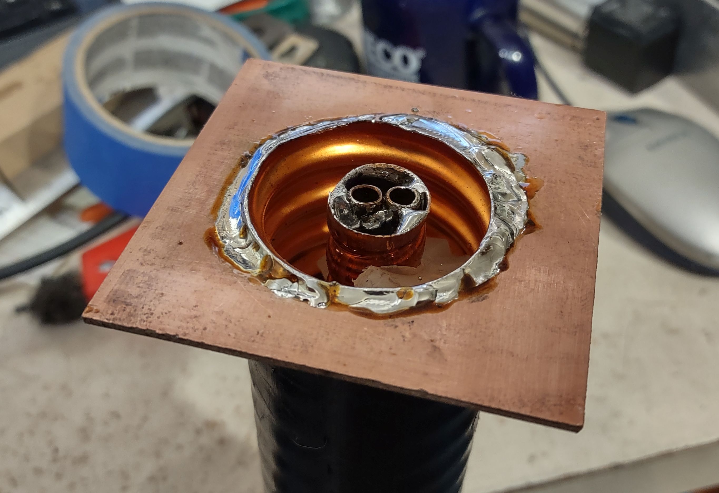
Figure 5: Three 0.1uF monolithic capacitors placed across the controller's terminals (C2a, C2b, C2c). Click on the image for a larger version.

 

Implementation

A glimpse of what was done may be seen in Figure 3.  Some 14 AWG paired copper wire (red/black) was wound on two FT140-43 ferrite toroids - about 6 bifilar turns in this case:  Individual wires could have been used other than "zip" cord - just be sure that the two parallel conductors are laid in parallel to maximize the effectiveness of the bifilar configuration.  Two of these wire/bifilar devices were constructed - one for the DC from the panel and the other for the output to the battery/load.  "Spade" lugs were installed on one end of the red/black wires - two lugs per wire/bifilar assembly.  (FT240-43 or FT240-31 toroids could also have been used, but the FT140-43 is a fraction of the cost, half the diameter, and perfectly suitable for this application.  The FT240 size may be more appropriate if such a filter network is constructed for a higher-current system with larger-gauge wire.)

On the solar controller itself, small 0.1uF, 50 volt monolithic capacitors were installed (C2a, C2b, C2c) to form part of the filter circuitry:  Minimal lead length is important for maximum effectiveness.  While monolithic capacitors are preferred because they are small (and will fit more easily in tight spaces) and have very low ESR (Effective Series Resistance) one could use disk ceramic capacitors instead.  Film/plastic capacitors are less effective at higher frequencies.

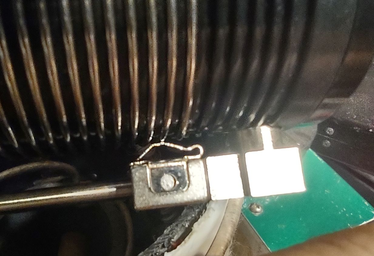
Figure 6: Terminal strip with capacitors C1a, C1b and C1c. As described, these capacitors do much of the "bypassing" of RF differential currents between the input and output. Click on the image for a larger version.

As can be seen from this picture, the terminals are the "clamp" type and are connected in the same manner as the lugs on the cable on the bifilar toroid assembly. - and also note that this "modification" is completely reversible as nothing at all was changed on the controller itself.

The other end of the red/black wires were soldered to a four-position screw terminal strip - similar to the one on the back of the charge controller.  As with the terminal strip on the controller, three 0.1uF 50 volt capacitors were soldered (C1a, C1b, C1c) on the back for RF bypassing.  It is possible to have connected the capacitors under the clamps as was done on the controller, but soldering them to the back means that they would not be prone to falling out or being lost if the cables were changed.

 

With these connections made, the wire on the toroids and the connections to the added terminal strip were covered with "Shoe Goo" - a robust rubber adhesive (used to fix shoes, as the name suggests) both as mean of strain relief and to provide electrical insulation.

 

The reader may have noted that we have physically brought together the input/output cables again at this terminal strip - and this was intentional.  By keeping the leads with the bifilar inductors as short as possible and then bringing them back together, we can use the shortest-possible leads on our capacitors to effectively "short" the input and output cables together at radio frequencies, making it impossible for the wires to radiate effectively at HF.  With this, the RF energy is contained within the area of the charge controller itself and the terminal strip/cables and since this is a very small aperture at HF, it can't radiate effectively and additional metallic shielding is unneeded.

 

At VHF/UHF frequencies - where the physical size of the controller+bifilar chokes is a larger proportion of the size of the wavelength (plus the fact that the components used won't work as well at these frequencies) means that some RF energy could radiate, but testing shows that the amount of VHF/UHF RF energy conveyed by the panel and cables was reduced below the point of detection more than a few feet (a meter) or so away from the system.

Spectrum analysis plots

Using a Tiny SA Ultra spectrum analyzer, I coupled the supplied telescoping antenna to the output (battery/load) cable by holding it in parallel with it.  While inductive coupling would have been preferable - and more repeatable and sensitive - this quick test gives a general indication of the nature of the energy being emitted by the charge controller and the reduction afforded by the added filtering.

Take a look at the "before" trace with no filtering:

Figure 7: "Before" (no filtering) analysis plot with the telescoping antenna of the analyzer held against the DC output cord. Click on the image for a larger version.

 

Figure 7 spans from DC to 30 MHz with each vertical division representing 5 MHz.  As can be seen, there is a peak of about -90dBm at around 7 MHz (40 meters) and several other peaks across the HF spectrum.

 

Figure 8 is the "after" trace with filtering:

 

Figure 8: The same plot/conditions as in Figure 7, except after the described filtering was applied. While it would have been preferable to have better-coupled to the wires from the panel/controller to measure the RFI, this wasn't done at the time in the interest of time resulting in the upper trace showing ambient (off-the air) signals and some local RFI rather than what the panels are producing. In tests with a portable radio, however, neither the panel nor the output cable (to the battery/load) carried any audible RF interference after the installation of the filtering. Click on the image for a larger version.

The JPC-12 antenna (possibly made by BD7JPC) is relatively inexpensive a portable vertical antenna - made in China, of course - that may be found for sale at quite a few places  under a few different brand names (including "Chelegance"). The price varies very widely - sometimes well over $200 - but I got mine via AliExpress for about $120, shipped, about a year and a half ago.

Note: 

I analyzed the JPC-7 loaded dipole antenna - which is made by the same company and uses many of the same components - and reported on it in previous article, and you may find that discussion HERE.

Stay tuned for a future article about rewinding/testing the loading coils of the JPC-12 and JPC-7 for better performance and lower loss.

Figure 1: All of the standard components of the JPC-12 kit. Click on the image for a larger version.

"The perfect is the enemy of the good"

The above statement should be kept in mind when doing any temporary, portable installation.  The idea is to have an antenna that will work "well enough" to do the job.  It's also likely that in the situation where you are portable, you will not (and cannot!) spend an inordinate amount of time tweaking things to eke out the last decibel.

This is not to say that one should not be mindful of good practices as too much corner-cutting can excessively impact performance and potentially replacing enjoyment with frustration.  One should achieve a balance between that which works well and something that will allow more operation than fussing about.

Remember:  The more time you spend trying to get that last bit of performance out of your system is less time that you are spending operating - and I'm presuming that operating is your goal.

What is included with the JPC-12

As shipped and as depicted in Figure 1, the antenna comes with these components:

• Aluminum ground stake.  This is a pointed stake 9-5/8" (24.5cm) long end-to-end about 1/2" (1.3cm) diameter.  This stake has M10-1.5 (coarse) threads on the end - the same as all other male and female threads used on the other mast/coil components of this antenna.
  

• Adjustable coil.  This is a piece of what appears to be thermoplastic or possibly nylon with molded grooves for the wire.  This unit is connected to the others via a male threaded stud on the bottom and female threads on the top, both being M10-1.5 like everything else.

Figure 3:  The adjustable resonator coil, wound with 1mm stainless- steel wire.  (The markings are mine.) Click on the image for a larger version.

The form itself is 4-1/2" (11.4cm) long not including the stud and 1-11/16" (4.3cm) diameter - wound with 34 turns of 18 AWG (1mm) stainless steel wire.  The coil has an inside diameter of approximately 1.66" (4.21cm) over a length of about 2.725" (6.92cm) and it has a slider with a notched spring that makes contact with the coil and this moves along a stainless steel rod about 0.12" (3mm) diameter that is insulated at the top, meaning that as the slider is moved down, the inductance of the coil is increased.

 

The coil has painted markings indicating "approximate" locations of the tap for both 20 and 40 meters when the telescoping section is adjusted as described in the manual using the four (originally) supplied mast sections.  The maximum inductance is a bit over 20uH and the DC resistance of the entire coil is about 4 ohms - more on this later.

• Telescoping section.  This is a stainless steel telescoping rod that is 13-1/8" (33.4cm) long including the threaded stud (12-7/8" or 32.7cm without) when collapsed and 99-11/16" (8' 3-11/16" or 253.2cm) when fully extended - not including the stud.
  

As with all stainless-steel telescoping whips, you MUST maintain them - keeping them clean and lubricated:  More on this later in this article.

Figure 4: This is the supplied "radial" kit - a 10-strand chunk of ribbon cable - the ring to be sandwiched on the bottom of the feed. Click on the image for a larger version.

• Counterpoise/Radial cable.  This is in the form of a chunk of 10 conductor ribbon cable terminated with large (0.4", 1cm I.D.) ring lug on one end sized to fit over the M10-1.5 threads.  This cable is about 203" (16' 11" or 516cm) long, including the ring lug that is intended to be sandwiched between the bottom of the coil and the ground stake. As noted later in this article, this radial isn't as useful/convenient/versatile as one might initially think.
  

• Padded carrying case.  This zippered case is about 14" x 9" (35.5x23cm) with elastic loops to retain the above antenna components and a zippered "net" pocket to contain the counterpoise/radial cable kit and the instructions.  There is ample room in this case to add additional components such as small-diameter coaxial cable - and enhancements to the antenna, as discussed below. 
  

• Instruction manual.  The instructions included with this antenna are marginally better than typical "Chinese English" - apparently produced with the help of an online translator rather than someone with intimate knowledge of the English language.  The result in a combination of head-scratching, laughter and frustration when trying to make sense of them.  Additionally, the instructions that came with my antenna included those for the JPC-7 loaded dipole as well, printed on the obverse side of the manual.

Fully assembled with the originally-supplied components, the length of the antenna is about 13' 5" (411cm) not including the ground spike meaning that it is self resonant - without added inductance - at a bit below the 17 meter band.  This means that at 17 meters and above, the tuning can be done solely with adjustment of the telescoping section and the coil can likely be omitted entirely.  Below 17 meters additional inductance is required which is obtained by moving the slider of the antenna downwards, requiring all but the last 3-4 turns of the coil to obtain resonance on 40 meters.

Comments:

Build quality

I'm quite pleased about the overall build quality:  The design seems to be well thought-out, perhaps inspired by other (similar) products on the market.  The individual mast sections seem to be plenty strong and I've seen no indication of the end sections coming loose.  I have screwed eight of these sections end-to-end and held them horizontal and noticed very little drooping and no "permanent" bends.

The feedpoint - being a combination of aluminum and plastic - seems to be well-built, the bottom section being machined with a flat to accept the SO-239 connector.  The upper section appears to be fiberglass, threaded at the top to accept an aluminum plug into which female threads are tapped to accept threads of the mast sections.

Likewise, the coil itself seems to be well built, the 32 turns of wire set into a spiral groove molded into the body with the coil tap selection having firm, positive action.  As noted previously, the wire comprising the coil is, itself, about 1mm diameter (approximately 18 AWG) and is apparently austenitic (e.g.  non-magnetic) stainless steel.

While this wire is very rugged, the fact that it is stainless means that its resistance is quite high compared to copper - in this case the end-to-end DC resistance is about 4 ohms - but the RF resistance, taking the "skin effect" into account, is likely to be very much higher.

Using Owen Duffy's online skin effect calculator (link) and assuming 1mm diameter, 316 Stainless, the 4 ohms of DC resistance translate as follows to RF resistance including skin effect:

• 3.5 MHz = 5.2 ohms
• 7 MHz = 7.2 ohms
• 14 MHz = 9.6 ohms
• 28 MHz = 13.6 ohms

While these values would be for the entire coil remember that less than full inductance is typically used  - but the message is clear:  The fewer turns of coil you need to use, the lower the loss!   The total length of 1mm wire is estimated to be about 180 inches (457cm).  By comparison, copper wire of this same diameter and length would have a DC resistance of about 0.1 ohm - or a skin effective resistance of 2 ohms at 28 MHz.  Alternatives will be discussed later.

Using the supplied radials - or not!

Noted in most reviews is the nature of the included radial/counterpoise wire - particularly since there is little or no mention of how it is to be used in the included manual.  Clearly, the single ring lug is intended to be captured between the bottom of the feedpoint section with the SO-239 connector and the ground stake.

For use as a resonant radial, the length of the this cable (203" or 516cm) is approximately correct for 1/4 wavelength at 20 meters, but this is not really suitable for 40 meters.  For best efficacy, the radials should be elevated above the ground by about a foot (25cm) or so so that the 1/4 wave impedance transformation (e.g. the distal end of the radial being open being transformed to a "short" at the antenna end to make it work effectively) but laying it on the ground directly - particularly if it is dry - will usually work quite well.

Being 10 conductor ribbon cable, the opportunity exists to split the wire lengthwise to obtain individual wires to spread radially around the base of the antenna.  This wire - with its PVC insulation and rather small gauge conductor (likely 26 AWG) means that it is difficult for it to lay flat unless it is warmed by the sun on hot ground (or with rocks laid on the wire) - plus a large number of connected-together conductors from a split-apart ribbon cable are the makings of a portable rats-nest of wires that cannot easily wound/unwound later.

Most reviewers/users of this antenna - including myself - don't really like the "ribbon cable radial" system and personally, I have never used it - but I keep it in the kit, just in case.  

Location of the loading coil

While it might be tempting to place the loading coil immediately above the feedpoint, this is not the suggested location, but rather at the top of the four supplied screw-together mast sections immediately below the telescoping section.  This makes sense on several counts:

• This elevates the coil above the ground, making it easier to adjust as it is at more convenient height (about 4' 3" or 130cm above ground).
  

• Because it is the portions of the antenna that conduct the most RF current are those that will radiate the most, those same sections below the coil - and above the connection to the counterpoise - will emit the bulk of RF energy
  

• The markings on the coil for 40 and 20 meters assume that you have placed the loading coil in the location described above using the original components in the kit.
  

From a practical standpoint, placing the loading coil immediately above the feedpoint will also work - albeit with some loss of efficiency - and this may be desirable if the base of the antenna (and radials) itself is elevated - perhaps by being clamping it to a fence post or table.  In this case one might place the coil closer to the feed point to keep it at a reasonable (accessible) height rather than needing to access the coil's tuning slider by standing on a ladder or chair. 

Augmenting/improving the JPC-12 with optional accessories

A bit of perusal among the goods of the various sellers of the JPC-12 (and the related JPC-7 dipole) will reveal that spare parts:  It's a pretty good idea that - if you find that you are using this antenna a lot - to get a few "extra" parts (I strongly suggest an extra telescoping section or two) when things inevitably get worn out or broken.  There are also several "accessories" that may be used with the antenna(s) that might be useful - some of which are discussed below - and other components that you can easily assemble and add to the kit.

Improved ground radial system

For a 1/4 wave vertical - and this antenna is exactly that, albeit electrically lengthened with a coil and tophad on the lower bands - half of the antenna is its mirror reflection from the ground.  As it is unlikely that most people will ever set up their antenna atop a metal surface or in salt water, a set of wires is typically deployed to locally simulate the needed reflective "ground" surface.

The common advice in years past has been to bury many, many ground radials just below the surface of the ground - advice that is practical in terms of avoiding trip-hazards and to provide a degree of lightning protection - equal or better performance may be had by deploying an array of radials that are odd-order quarter-wave multiples (1/4, 3/4, 5/4, etc.) that are elevated slightly above the ground.  Emperical testing (see the linked article below) that as few as three or four elevated, resonant radials can be quite effective - and this number of radials is perfectly manageable in a portable installation.

The accessories described below make it easier to quickly deploy a resonant ground radial system - elevated or not.

The ground radial plate 

Figure 5: This is the "radial plate" - an add-on accessory.  Spade-lug terminated radial wires connect easily under the wing nuts. Click on the image for a larger version.

As shipped, the radial kit (ribbon cable) included with JPC-12 antenna is perfectly usable - but in the opinion of many (including myself) the supplied radials aren't particularly practical or convenient.  From the same seller as the antenna I purchased what is cryptically called a "JPC-12 PAC-12 Network Disk" - seen in Figure 5.

What this really is is an aluminum disk about 4-3/4" (12cm) in diameter with a series of eight wingnuts and screws around the perimeter with a center hole sized appropriate for the M10 stud on the top of the ground rod or one of the antenna elements.  This device makes the connection of individual ground radials equipped with spade lugs much more convenient.

In looking at Figure 5, you may have realized that it's sitting atop its protective pouch to keep the screws from tearing up the inside of the carrying case:  The rear pocket removed from an old pair of blue jeans!

Using individual wires for the radials

Figure 6: Four radials on kite string winders - each long enough for 60 meters - with markers on the wires for the different bands. Click on the image for a larger version.

Rather than using the original ribbon cable, I have four lengths of 22 AWG hookup wire on kite string cable winders (a pack of ten cost US$10 from Amazon - including the string!)  These four wires are terminated with spade lugs to slide under the screws on this pate and are each 44' (13.4 meters) long corresponding with the quarter-wavelength at 60 meters.

Marking the radials' lengths

At various points along the length of each of these wires are pieces of marked heat-shrink tubing to indicate the points corresponding to quarter-wavelengths of the various amateur bands from 60 through 10 meters and only as much wire as needed is unspooled from the cable winder to achieve the desired length for the intended band of operation:  These yellow tags can just be seen in Figure 6 among the wire on the winders.

For these marker tags I used heat-shrink tubing cartridges for my Brother label maker - but I could just have easily have written on  light-colored tubing with an indelible marker prior to shrinking them.  To keep these tags from sliding around I put a dab of "Shoe Goo" (rubber repair adhesive) on the wire and slid the tubing over it before applying heat, locking it into place with much greater tenacity than the compression of the tubing shrinkage alone:  Having used these radials in the field a quite a few times, I have yet to have one come loose.

Using elevated radials

From an operational standpoint, just three or four elevated, resonant radials will perform equally to or better to a large number of radials - resonant or not - buried in the ground.  The reason for this - alluded to earlier - is the fact that any open-ended conductor that is an odd multiple of a quarter-wavelength long (e.g. 1/4, 3/4, 5/4) will exhibit a low impedance on the opposite (antenna) end - which is exactly what we want.

Simply laying such a length on the "average" ground will tend to diminish this effect somewhat, but elevating it even a short distance above the ground will preserve it.  For more information and an analysis of vertical antennas with elevated radial systems see the article "A Closer Look at Vertical Antennas with Elevated Ground Systems"  by Rudy, N6LP - LINK.  It's worth noting the admonition of the author of this page to avoid the use of radials that are around 1/2 wavelength long and multiples thereof - likely for the reason that the nature of a free-space half-wavelength conductor is not to provide a low-impedance on their proximal end when the distal end is unterminated!

The obvious hazard of elevated radials is that of tripping - of you, the operator, others in the area, or animals, so it isn't necessarily practical in every situation.  If it is possible to control access to the area with the antenna - or raise the radial above the height of the average person for much of its length - then this is a good choice.

Figure 7: Fiberglass driveway markers modified to mark/hold radials. Click on the image for a larger version.

In my operation - typically out in isolated areas - I don't have much worry about tripping anyone other than myself so I obtained some 4' (1.2 meter) long fiberglass driveway marker stakes.  These bright-orange stakes are about 4" long each (122cm) each - much 1--  long to fit in the antenna case, so eight of them were cut to shorter lengths to allow them to fit in the case, yielding two pieces each - the bottom portion with the sharpened point cut to 11-3/4" (30cm) and the top portion cut to 13-3/8" (34cm).  To the bottom portion, I glued (again using "Shoe Goo") a 2" (5cm) long of 8.5mm I.D. stainless steel "Capillary" tubing (found on Amazon) so that the two pieces could be assembled to a single (mostly) non-conductive post about 26" (66cm) long.

Eight of these two-piece posts allow the support of four elevated radials at two points along their length, the radial wire being wrapped once or twice around to form a friction fit to keep them from sliding down.  At the distal end, the remaining lump of wire still on the kite string winder is simply wrapped and hung over the post once a slight amount of tension is pulled on it.

Figure 7 also shows something else:  I made a drawstring bag (again, from an old pair of blue jeans) that keeps all of these post pieces together and it can accommodate some of the extra mast sections, all while fitting in the original padded antenna case.

Comment: 

The reader should be conscious of the fact that for the purposes of this discussion, we are talking about a temporary, portable antenna rather than a permanent installation.  In the case of the latter, a different approach (the deployment of many, many radials, perhaps buried) is reasonable - but for a temporary antenna - where less effort to erect and break down is desirable - the use of four elevated, resonant (e.g. 1/4 wavelength) radials is likely to outperform the same number of radials laid atop the ground.  In either case, however, the antenna will be usable - and that's the entire point!

On-the-ground radials

The use of elevated radials is arguably most important on the lower frequencies of operation of this antenna - namely 40 and 30 meters - where efficiency of this "electrically small" antenna will suffer due to a number of factors, but maximizing the efficiency of the ground plane is one way to mitigate this.  In those cases where it is not practical to elevate the radials, the wires may simply be laid atop the ground.  

As these posts are intended for marking driveways they are bright orange, making them stand out, but near the top they have a piece of white reflective tape so that they will show up at night.  As I had this type of tape on hand I added a piece to the bottom section as well - just below the stainless steel capillary tube - to make them even more visible - particularly if the bottom and top portions are used separately to mark where an on-the-ground radial might be run to warn against a possible trip hazard.

The use of a "Magic Carpet" (e.g. "Faraday Fabric")

There is no reason why one could not use the aforementioned conductive fabric as part of their ground plane - but you would probably have to construct an additional component to connect to the fabric and use it effectively.  For this, a piece of clean aluminum or copper plate laid atop the fabric - possibly weighed down with a rock - should provide a low-impedance connection to it.

While I do own some of this "Faraday Fabric" (obtained from Amazon) I have yet to try it with this antenna - and when I do, I plan to perform an "A/B" comparison.  As of the time of this writing I have yet to see a serious, scientific and well thought-out comparison between a simple radial field and the use of just the fabric:  Most of these comparisons simply demonstrate that it is possible to get a good antenna match while using the fabric - but as we all know, simply getting a match does not mean that the antenna will work:  After all, a dummy load has a great match!

I expect that - at least on the sort of desert ground that I'm likely to encounter - the radials will "win" the contest - although I still plan to do a comparison:  I suspect that using both the fabric and radials will offer decent results - even when tuned to a higher band for which the lengths of the radials are not expected to work (e.g. 20 or 10 meters with 40 meter radials.)

Additional antenna height - both real and "virtual"

Figure 8: The accessory top had kit consisting of a machined piece that attaches to the top of the vertical with four telescoping rods. Click on the image for a larger version.

Any antenna that has to be electrically lengthened with inductance is likely to suffer from efficiency loss as that inductor is unlikely to be comparatively lossy.  As the antenna is mechanically "about" 1/4 wavelength on bands above 20 meters, it make sense, then, that the lower bands that it is intended to cover - particularly 30 and 40 meters - need some additional inductance to bring it to resonance.  It further follows that anything that may be done to make the antenna "taller" will reduce the amount of needed inductance and minimize these losses.

Tophat capacitance

Another accessory available for this antenna is a small tophat attachment for the telescoping vertical section.  Often described as a "PAC-12 Capacity Cap" this consists of what looks like a knurled aluminum knob with five holes drilled around its circumference and yet another hole on the bottom sized to receive the "static ball" (really a short cylinder) atop the telescoping section.

Using a set screw to secure it to the top of the antenna, this kit contains four small telescoping whips (3-1/8" 8 cm long collapsed, 12-1/4" 31c fully extended - not including threads) that screw into the 5/8" (2cm) diameter center disk.  Assembled, the end-to-end length of two of the telescoping elements is 25" (98.4cm) which forms a four-spoke "disk" that adds to the effective height of the main telescoping section of the antenna by increasing the capacitance.  The idea (and hope) is that this allows the reduction of the amount of inductance needed to bring the system to resonance - and it also allows potential coverage of 60 meters as noted later.

The size and weight of this attachment is, in my opinion, about right:  Any larger or heavier, it would likely be too much for the fully-extended main whip to handle and expose it to excessive wind loading.  To be sure, one must always be very careful when handling the whip when fully-extended, anyway and adding the tophat increases the risk of damage.

Figure 9: The top hat kit assembled - but the rods are not extended. Click on the image for a larger version.

Testing has shown that the addition of the tophat - when the antenna has previously been tuned for 40 meters - lowers the resonant frequency by approximately 1 MHz indicating an increase of virtual height by about 12 percent at that frequency.  Even with the tophat the antenna falls short of being able to resonate at any 60 meter frequency with the normal complement of parts included with the antenna.

For the higher bands, the top-hat may be enough to eliminate the need for the coil on 20 meters - or at least greatly reduce the amount of coil and thus the potential loss.

Of course, the use of this top hat means that the existing coil marking scheme (e.g. the paint marks that show approximate slider position for the bands) is meaningless as tuning is changed - but if one is already prepared in the field for this (e.g. using an antenna analyzer, added markings to the coil for the new configuration, a paper template marked with pre-determined coil positions) then this is of little consequence.

This tophat kit is constructed fairly well, using a small grub screw with a supplied Allen key to attach it to the top of the telescoping section, but I noted that the key and the screw weren't well matched and couldn't be tightened too much with the key slipping.  Rummaging about in my collection of hardware I found several metric machine screws and a hexagonal brass stand-off with matching threads and I replaced the grub screw with the stand-off, allowing it to be attached firmly to the top of the telescoping section using just my fingers.

Additional mast sections

It should not be surprising to know that you can buy individual mast sections.  These are often described as being "dedicated lengthened vibrator for JPC-7 (PAC-12) multiband portable antenna".  I purchased two more of these sections when I first purchased the antenna, increasing its fully erect height from 13' 5" (411cm) to 15' 7-5/16" (476cm) and coupled with the tophat and the full inductance of the coil allows the antenna itself to resonate at approximately 4.7 MHz, allowing complete coverage of the 60 meter band.

Figure 10: Four more mast sections to be used in a variety of ways - as ground supports, or as the "live" mast itself. Click on the image for a larger version.

At this extended height and with the tophat, this antenna was used in fairly high winds with gusts of 35 MPH (approx 67 kph) with no issues:  Having clamped the ground stake of this antenna to a metal fence post helped keep the antenna vertical and minimize sway certainly helped!

After using the antenna several times, I purchased yet two more mast sections (for a total of eight) - not only to have as spares, but also to elevate the bottom of the antenna still further.  Living in the desert west of the U.S. (Utah) it's often the case that there is only sand into which the ground stake can be pushed and it simply isn't long enough to adequately support the antenna:  Lengthening the ground rod with the addition of another mast section allows the ground stake to be pushed in farther and support the antenna without burying the feedpoint below ground level or stealing one of the mast sections from the antenna and reducing its height.  This is mostly a problem on the lower bands (40 and 30 meters) where one needs as much height as one can get to maximize antenna efficiency.

This extension also facilitates the use of an elevated ground radial system, placing the feedpoint - and the ground radial disk - at a reasonable height.

Maintenance

The telescoping whip(s)

The telescoping whip is certainly the most fragile component included and it - like any other telescoping antenna - is easily broken if one is not careful.  The "safest" way to collapse one of these things is to pull it down - section by section - starting from the bottom:  One should NEVER push it down from the top as that is just asking for problems.

As with any telescoping whips that I own, one of the first things that I do when I get it is to make sure that it is clean of dirt and oxidation (particularly if it has been "pre-owned") as this can cause the metal-on-metal - especially when the two metals are the same - to gall and seize up, making it more difficult to extend or collapse.  If I do find a section that is hard to move, I carefully examine it, often discovering slight scratches, buffing them out with very fine sand paper (1000 grit or finer) and/or steel wool (size 0000 or finer).

The final step - after cleaning with paint thinner or alcohol to remove any dust - particularly if it was just buffed with steel wool or sandpaper - is to put a light coating of oil on all sections when they are fully extended:  I prefer to use a PTFE ("Teflon") based lubricant like "Super Lube" (made by Synco) as it does not dry and become "gummy".  Extending and then retracting the whip a few times does a decent job of spreading out the lubrication - even getting inside the individual sections.

Although much smaller, I did a similar thing to the four telescoping whips that comprise the tophat.

I would consider this "cleaning and lubricating" to be a necessary maintenance item when using this antenna, needing to be done occasionally, with constant vigilance toward possible issues every time it is used.

Inductor slider

The adjustable inductor's components are all stainless steel - including the coil wire itself.  Besides being known for the fact that this material "stains less" than others, it is also known for galling - that is, developing tiny burrs on the surface and jamming up when it is used against the same type of metal:  In the case of stainless screws, nuts and bolts - if these gall, even if you ARE able to remove them without breaking them, they have to be replaced.

While the contact area on the slider is small enough that it is unlikely to gall and get "stuck", I noticed immediately a bit of "roughness" in its movement that indicated excessive metal-on-metal friction:  I could not tell if this was on the contact area of where the slider rubbed across the coil's windings or on the sliding rod itself - but it was probably a combination of both.

This "roughness" in movement was relieved with the application of lubricant - the same "Super Lube" used on the telescoping sections - also making the adjustment easier to do.

Improving the coil

As noted previously, the coil is wound with 18 AWG (1mm dia) stainless steel wire.  It is suspected that one of the main reasons why this type of wire is used despite its terrible losses - as compared with copper - is that this resistive loss increases the feedpoint resistance - but at least in relatively cool temperatures (below 90F or 32C) I wouldn't worry about running key-down for several minutes at 100 watts - or higher power with a low duty-cycle mode like CW or FT-4.

As it happens, one can juggle the proportions of a vertical antenna a bit to vary the feedpoint resistance - but if you consider that these same coils are also used in the JPC-7 dipole, the reasoning behind the use of stainless steel wire becomes more clear.  An electrically-short dipole - such as when the JPC-7 is configured for 40 meters - would ideally have a feedpoint resistance of just a few ohms - but this would not match at all well to a 50 ohm system:  Even a very low-loss antenna tuner would have difficulty coping and placing the tuner away from the antenna through a length of coaxial cable would make the situation even worse!

Having said that, testing was done that revealed that on the JPC-17 - while operating on the lower bands (30, 40 meters) a significant amount of power was being dissipated in the coil - enough to raise its temperature by 135F (75C) at 70-100 watts on 40 meters (lower loss on higher bands) - but rewinding the coil with silver-plated copper wire pretty much eliminated that element of loss.

A future article on this blog will detail the rewinding of this coil along with measurements/comparisons between the original stainless steel and rewound coil for both the JPC-7 dipole and this JPC-12 vertical which will eliminate any nagging worries about power handling capability.

Using the JPC-12 vertical in the field

I have used this vertical in the field a number of times, mostly with the "augmented" kit with the extra mast sections, top hat and ground radial plate and elevated radials - typically on 40 and 60 meters SSB, but also for POTA using CW.  While the signal reports comparing my signal with that of others using full-size antennas unsurprisingly indicates that this doesn't to as well as the others on the lower bands, conditions have generally been good enough that there was little difficulty in copying my signal.

Figure 11: The JPC-12 vertical out in the wild in a slight breeze. The tophat is installed as is a section below the radial plate - along with extra sections to increase height. Click on the image for a larger version.

As the ground here in Utah is usually rather poor making it difficult to simulate the "other half" of a vertical antenna, it is even more important that the radial system be effective.  While I usually configure it to have four radials elevated about 18" (0.5 meters) above the ground, I have also simply laid the radial directly on the sandy soil - or found some convenient sagebrush, scrub oak or some other low plant or small tree to support them off them ground - and have always had pretty good results.

While I like this antenna, I find it to be far less convenient than the JPC-7 loaded dipole in that the vertical takes quite a bit more time to set up, needing a bit of assembly of the various pieces and laying out of the radials.  With resonant radials, changing bands - and trying to maintain optimal performance - also makes it a bit awkward by the fact that the radials need to be shortened/lengthened as appropriate/

Practically speaking, having the radials laid out for 40 meters and running on 60, 30 or 15 meters isn't much of a problem, but picking a band that is an even multiple of the radials' base resonant frequency - being an odd half-wave multiple (e.g. 20 or 10 meters with a 40 meter radial) - will not work well as that is the worst possible radial length (other than zero length) to choose:  The half-wave length will not provide the low impedance at the antenna and it's also likely that the coaxial cable will become most of the radial, possibly causing a "hot rig" in terms of RF and the related ill effects (RF into the audio, computer/radio crashing, extra noise) from doing so.

If, however, I have a bit of extra time and I want a better signal that I would otherwise get from the loaded dipole or a mobile-mounted HF antenna, I would definitely set up the JPC-12.

* * * * *

Comment:  I analyzed the JPC-7 loaded dipole antenna - which is made by the same company and uses many of the same components - and reported on it in previous article, and you may find that discussion HERE. 

This page stolen from ka7oei.com

[END]

Comment:

This article - while it centers about the investigation of a SolarEdge PV (PhotoVoltaic) system - the discussions of techniques and strategies should be generally useful when investigating interference from any make or model of PV system - or even interference from other sources.

* * *

Several months ago I got a call from a local amateur who was very concerned about a sudden rise in his noise floor across the HF spectrum (3-30 MHz).  This increase in noise seemed to be coincident with the installation and commission of a 5 kW PV (Photovoltaic, or "Solar") electrical system on the house of an adjacent neighbor.  I suggested that he talk to the manufacturer of the PV system to discuss the situation - and to request from them possible solutions.

A few weeks ago, he got back to me and he had, in fact, talked to the manufacturer and an online meeting was arranged in which they would remotely idle the neighbor's system while we were monitoring via the amateur's receive antenna.

Out of curiosity - and as sort of a practice run - I went over the weekend before the online meeting to get a better idea as to the spectral signature of this system - a SolarEdge series string system with optimizers - when it was operating normally.  The amateur had obtained permission from the neighbor to allow us to enter their yard to make very "close in" measurements (e.g. within a few inches/cm of the equipment, conductors) to obtain spectral "samples" of the system, thereby excluding external signals.

For these measurements, I used an amplified, shielded magnetic ("H") loop antenna (about 18"/50cm) in diameter as the "sense" antenna and an HP/Agilent/Keysight spectrum analyzer, recording the plots electronically - although a Tiny SA "Ultra" would likely have sufficed as well.  None of the readings were to represent "absolute" signal levels as all that we were really interested in were relative measurements, and as such all that we needed to do was keep our measurements consistent - that is, being able to precisely repeat the conditions between subsequent measurements.  These readings would allow us to understand the nature of the RF energy that it was creating - its "signature", if you will.

Note:  For information about the H-field loop used for this testing - and using an inexpensive spectrum analyzer such as the "Tiny SA" or, better yet, the "Tiny SA Ultra", see a previous blog entry "RFI Sleuthing with the Tiny SA" - Link.

The nature of this QRM:

The interference observed by this amateur - now known for certain to be signature of this model of SolarEdge PV system - was evident as two general types of signals:

• Moderate to strong clusters of carriers every "even" 200 kHz.  At 200 kHz intervals (e.g. 7.0, 7.2, 7.4 and 14.0, 14.2 and 14.4 MHz) from below 3 MHz through at least 30 MHz could be heard a melange of closely-spaced carriers within about 500 Hz of each other on the lower bands.  While these carriers sounded like mostly CW (unmodulated) signals, there was also evidence of low rate data signalling buried in the cacophony as well as additional lower-level carriers.
  

While the appearance of the above interference coincided with the activation of the neighbor's system, that fact that it disappeared at night further pointed to a PV system as the source of the QRM.

"Close-in" measurements

Placing the sense antenna right at the main inverter on the back of the neighbor's house, we wanted to take a snapshot of the spectrum at that location:

Figure 1:  0-30 MHz sampled right at the main inverter

With each horizontal division representing 3 MHz, this 0-30 MHz plot shows a high concentration of noise in the 3-9 MHz area from a location right at the inverter.

Because Figure 1 represents the spectrum at the inverter, we wondered what it would look like at one of the solar panels so we placed the sense antenna right against one of the solar panels:

Figure 2:  0-30 MHz sweep with sense antenna placed next to a solar panel

Figure 2 is in the same frequency and amplitude scale as Figure 1 - but with the "reference level" adjusted by 20 dB to move the trace "up" a bit - and we can see that the spectrum next to the panel looks quite different from that sampled right at the inverter.  This isn't unexpected as Figure 2 would likely represent more of the noise that is emitted from the DC (input) side of the optimizer whereas the spectrum represented in Figure 1 would be more likely to show that of the DC output of the optimizer plus whatever noise was riding on the conductors carrying the DC input and AC output of the main string inverter.

Although it is difficult to be sure, the 0-30 MHz plots taken from a greater distance (10 meters or more) had the general appearance of the noise spectra shown in Figure 2 more than that of Figure 1 leading me to believe that a significant portion of the QRM may be being radiated from the panels themselves rather than just the conductors going from the optimizers  to the main inverter - but certainly, both are likely involved.

Note:  For both of these plots, the RF energy from the PV system was many 10s of dB above the typical background noise floor - in this case, 40-50dB for Figure 1 and at least 30dB for Figure 2 in the area around 7 MHz.

As the 0-30 MHz sweep does not have enough resolution to visualize the narrower 200 kHz signals, the analyzer was readjusted as depicted in Figure 3 - again with the sense antenna next to the panel:

Figure 3:  From near the panel, a "zoomed in" spectral sweep showing narrowband birdies.

In this spectrum plot we can see not only the "white" noise on the floor of the sweep representing the "hummy hiss", but also the much stronger signals every 200 kHz - plus a number of weaker signals in between:  It is these signals that are the most obvious to the casual operator and appear to be unique to a SolarEdge system of this model/type.

On this same day we waited until after sunset - monitoring the groups of carriers at 7.2 MHz and hearing them "flicker" out of existence as it got dark and we re-did the "next to the panel" measurements - this time the spectrum was devoid of the 200 kHz-spaced carriers (they were no longer audible on the amateur receiver, either) and the 0-30 MHz plots were 10s of dB lower than in the daylight. 

Important:  The 2 MHz sweeps in Figures 3-7 use a resolution bandwidth of 10 kHz which is almost exactly 4 times wider than the typical SSB bandwidth of an amateur receiver of about 2.5 kHz making their apparent level above the background noise appear lower than it is actually is.

What this means is the coherent signals - such as the 200 kHz carriers - appear to be another 6 dB farther above the noise floor in an SSB bandwidth than what the analyzer plots show.

Plots from a distance

Having captured some "close-in" plots, we now had an idea as to what the signals emitted by the PV system looked like.

A few days after we made the above plots we were in a virtual meeting with the manufacturer of the PV system (SolarEdge) from the ham's shack.  Having reconfigured the feed to his main radio, we could quickly switch the feedline from the antenna feeding the radio and the spectrum analyzer.

At this time we also learned that there was a second SolarEdge system south of this amateur's QTH - about 150 feet (45 meters) away across the cul de sac - and that the neighboring system and the one across the street would but remotely shut down, in that order, to determine how much QRM was emanating from each.

While we captured 0-30 MHz plots of each stage of system shutdown, for the purposes of this article we'll show just the "narrow" plots in 2 MHz sweeps as depicted in Figure 3 as the presence of the 200 kHz signal are generally representative of the presence of the broadband noise as well and these signals were easily identifiable and now known to be indicators of QRM from this type of PV system.

First, here's the plot from the amateur's 40 meter inverted Vee antenna with both systems on:

Figure 4:  6-8 MHz plot from the 40 meter antenna showing the 200 kHz peaks - and a bit of broadband noise as well.

 

The next plot shows the effects when the neighboring system was turned off, but the one across the street still on:

Figure 5:  The neighboring system off - but the one across the street still on.

As can be seen, the broadband noise floor around the 40 meter band (approximately one horizontal division below and above the marker) has dropped visibly - around 3-4 dB - and the amplitude of the carrier at 7.2 MHz has dropped about 6 dB - and the 200 kHz signals have disappeared almost entirely below about 6.5 MHz.  The system across the street was then shut off and the only remaining signals were those that happened to be on the 40 meter band.  (No trace is available for this configuration, unfortunately.)

As the 40 meter inverted Vee is oriented to favor east-west signals it was not necessarily the best candidate to test the effects of the PV system across the street, so we switched to a 20 meter antenna which was responsive in that direction and this trace shows the plot between 13 and 15 MHz:

Figure 6:  This plot of the 20 meter band and surrounding frequencies shows only propagated signals, with no sign of PV system QRM.

As both systems were off, the trace was quite clear - only showing signals that actually were on or near the 20 meter band, propagated from elsewhere in the world.  The folks at SolarEdge then turned on the system across the street with the following result:

Figure 7:  Same as Figure 6, but with only the PV system across the street activated.

The effect is clear:  In the vicinity of the 20 meter band, the appearance of rather strong signals every 200 kHz is apparent - and there is an obvious 2-4 dB increase in the noise floor indicating that this system, too, is causing harmful interference.

Readings on the radio:

It would seem that the folks at SolarEdge had worked with more than one amateur radio operator on similar issues and I was pleasantly surprised when they asked for some "S-Meter" reading comparisons with the neighbor's system on and off.  Using a calibrated signal generator, I'd already determined the signal level (in dBm) that correlated with the S-meter readings for the Icom radio - and here are the results for 40 meters:

Both systems off:

S1 (<= -84 dBm) - no carrier groups every 200 kHz.

Neighbor system on:

S4 (-78 dBm) - white noise between 200 kHz carriers.

S9 (-67 dBm) - carriers at 7.2 MHz.

This shows that at 40 meters, the degradation to noise alone was on the order of 6 dB (most Japanese radios are calibrated for 3dB per S-unit) and that the cluster of carriers on 200 kHz intervals was far more destructive, rising a bit short of 20dB out of the noise floor.

As our time with the SolarEdge folks in the virtual meeting was limited, we were not able to do similar "S-meter" tests on 20 meters, but we can use the 40 meter results along with the relative strength of the 200 kHz-spacing carriers  and correlate them with the 40 and 20 meter spectrum analyzer traces and determine that the severity of QRM from the PV system on 20 meters on the receiver would have been roughly comparable to that on 40.

Analysis of these readings and implications:

As mentioned earlier, there are two types of interfering signals produced by these SolarEdge PV systems:

• Moderate to strong clusters of carriers every "even" 200 kHz.  These are very obvious, easy to identify, and quite strong compared to the noise with a few weaker signals in-between that were also clearly audible.
  

The RX-888 (Mk2) and external clocking

Figure 1: The RX-888 with external clock input (right) The enable/disable switch is barely visible behind the USB connector. Click on the image for a larger version.

• Improving the thermal management of the RX-888 (Mk2) - link - This page talks about highly recommended modifications to the RX-888 to reduce internal heat to improve reliability.
  

• Measuring signal dynamics of the RX-888 (Mk2) - link - This is a discussion of how much (and little) signal is needed to stay within the dynamic range of the RX-888 and the effects of gain and attenuator settings.

Adding an external clock connection

While the internal 27 MHz TCXO in the RX-888 (Mk2) is pretty good, there may be instances where one wishes better accuracy and stability.  Fortunately, the RX-888 (Mk2) has provisions for doing so in the form of a jumper to disable the internal clock (when the jumper is removed) and a small connector (a tiny U.Fl) on board to accept that clock.

Unfortunately, it is up to the user to add the cable to feed an external clock - but short 4-6" (10-15cm) cables already fitted with a U.Fl male and SMA chassis-mount female connector are easily obtained from the likes of Amazon, EvilBay and others - just be sure that you do NOT get a "Reverse" (RP) SMA by mistake!

This leaves the jumper.  While many people simply remove the jumper and mount the external clock connector between the HF and VHF inputs - or sometimes to the right of the USB connector knowing - from then on - their RX-888 will be unusable unless there is an external clock input - I prefer to make use of the ability of the internal clock to be switched - using (ahem) a switch allowing for testing/use of the RX-888 in a "stand alone" configuration - but this is up to you.

If one is careful, it's possible to mount the external clock SMA connector and switch on the same panel as the USB connector, orienting so that its handle is toward the "Clock In" connector to indicate that an external clock is to be used - but labels or markings are always nice, too!

If one takes the route of mounting the external clock input between the HF and UHF inputs, the switch could be placed to the right of the USB connector - or, if as in the case of one of my RX-888s where I put a heat sink on the FX3 chip and there wasn't room there - I found a very small toggle switch that just fit between the case screw and left side of the USB connector and tip of this switch may be spotted just behind the USB connector in Figure 1, above.

IMPORTANT:  As the external clock input is simply wired in parallel with the internal 27 MHz clock.  What this means is that with the internal clock enabled, it will be present on the external clock input.  Similarly, if you supply a 27 MHz external clock without disabling the internal one, the two will "fight" each other and you'll get "garbage" results.

What type of signal to use as an external clock

• The best external clock source is a 27 MHz sine wave of between 1.25 and 3.3 volts peak-to-peak.
• A series coupling capacitance of between 100pF and 1000pF (470pF typ.) should be present on the "center pin" between the RX-888 to eliminate a DC path to ground on the signal line.
  

While a capacitively-coupled 27 MHz sine wave is recommended for reasons that will be mentioned later, a lot of devices offer square wave outputs - and getting these to work reliably requires at least a little bit of attention.

Using the Leo Bodnar Precision GPS Clock to drive an RX-888:

Because the RX-888 natively requires a 27 MHz clock this means that if you already have a 10 MHz standard (GPS, Rubidium, etc.) kicking around, you will not be able to use it directly.  While it's not too difficult to synthesize 27 MHz from 10 MHz (a number of Si5351-based devices can do this) it's most common for users of the RX-888 to use a device such as that sold by Leo Bodnar, which can be programmed for almost any frequency (from audio through UHF) with good precision and accuracy.

You can look at these products here:  https://www.leobodnar.com  (I have no stake in Bodnar, but I have used them and I and others have had good success.)

The most commonly-used device is the Bodnar "Mini" - which has one output - and this single output is often "daisy-chained" between RX-888s.  There is also the functionally similar LB-1420 with a single output and the "Precision GPS Reference Clock" which has two signal outputs - but there is very limited ability to set the "second" output to a specific frequency and it's mostly useful for outputting the same frequency on the two ports - or outputting a 1PPS signals on the "unused" port.

Testing with a square wave - such as that produced by the Leo Bodnar GPS reference revealed that the drive level was far more finicky - and this has to do with the fact that a "square" wave with a reasonably fast rise time does NOT remain a square wave for very long as it quickly turns into something rather spiky and distorted as depicted in the image below:

Figure 2: A typical square wave output from a Bodnar GPS reference at the end of about 3 feet (1 meter) of unterminated cable.  Ringing is evident!

With multiple "spikes" that can occur on such waveforms due to distortion, it's possible - even likely - that certain combinations can result in multiple triggering peaks of the waveform.  In an extreme case, such distortion can cause the Si5351 to be triggered at twice the actual clock rate - but rather the result may be instability resulting in the RX-888 clocking which can be manifest as anything from no signals being "present" to those that are being off-frequency, varying, or just "noisy" - and this errant behavior may vary with temperature and slight changes in operating voltage.

It's important to realize that like the RX-888, the Bodnar is ALSO DC-coupled which explains why the above waveform in Figure 2 largely rests above the center line (zero volts) with the exception of some "ringing" which extends negative and is likely being clamped somewhat by the '888's internal diodes.

With a 3.3 volt waveform emanating from the Bodnar, we can reasonably expect that - if the signal isn't too "ringy" that a signal exceeding about 1 volt positive just once per cycle is likely to trigger the 888's Si-5351 correctly.

IMPORTANT:  If you try to directly drive an RX-888 with the output of a Bodnar, it will probably NOT work reliably!  I have observed this with my own Bodnar/RX-888s and many others have reported the same issue.

Remembering that the external clock input of the '888 goes directly to very sensitive logic devices, a simple resistive attenuator pad will do double duty:

• Rather than a very high impedance circuit that has a low resistance path from the outside world to a sensitive logic gate, resistance to ground offers a degree of protection by offering a relatively low resistance to ground and the series resistance provides at least some limit to input currents.
  

• While theoretically OK, the output of the Bodnar will not reliably drive the input of the Si5351 in the RX-888 directly, but being reduced to half or third of its original output seems to be pretty reliable and is less likely to cause clipping of diodes on the input circuit which can exacerbate ringing and other types of waveform distortion.
  

A 6 to 12 dB resistive pad - either 50 or 75 ohms - is a reasonable choice offering a bit of voltage reduction - but staying well above the 1 volt usability threshold - and such a pad, even if it is not connected to a 50 ohm load, will provide a bit of resistive termination, likely reducing the tenacity of reflections.  While a resistive pad does not offer DC decoupling between the center pin of the '888's external clock input, it works with the Bodnar as that device sources a square wave referenced to zero volts so the pad simply acts as a voltage divider for that square wave.

Testing has shown that the '888 seems a bit more forgiving of signal drive levels if there is a DC blocking capacitor on its signal input - something that could be provided by placing a "DC block" device (available in SMA, BNC or F-type connectors) between the '888 and the external clock source.

Caveats and warnings - and why the '888 is so finicky about its external clock

The external clock input of the RX-888 - as described in better detail in the next section of this blog post - is connected DIRECTLY to inputs within the '888 and as such, it has a few undesirable properties:

• There is a DC connection between the external clock, the oscillator output and the input to the 888's internal Si5351 synthesizer.  This exposes the clock input directly to extremely static and voltage-sensitive inputs.
• Because of this, it's very easy to damage the RX-888 when using and external clock, particularly if there are voltage potentials between different pieces of equipment.

• There is diode clamping between ground and the 3.3 volt input.  In the '888, this is primarily a BAT99 dual diode, but it also includes the protection diodes of the other devices in the circuit - namely the output of the onboard 27 MHz oscillator and the input of the Si5351 itself.  At first this might seem like a good thing - and it sort of is - but this means that any signal input to the RX-888 should be capacitively coupled - or directly to a 0-3.3 volt signal.  This is one aspect of the '888 that was definitely not well considered or implemented.
  
• What this means is that if you try to drive the RX-888's clock input with a source that is DC "grounded" - which includes devices that are transformer-coupled (e.g. a splitter to send the clock to multiple units) that the voltage output will be bipolar.
• For example: 
• If you were try to use a T1-1 isolation transformer to break a ground loop between the external clock input and the Bodnar - as well as other devices - the signal input may be 3.3 volts - but bipolar - that is, it will go above and below "ground" by about 1.65 volts - but since there is diode clamping, the negative-going signal will distort the waveform.
• The result of this can either be finessing required to find the precise drive level to make it work at all or - sometimes - you will find the signals at the wrong frequencies (sometimes at about half the expected frequencies) if the badly-distorted waveform triggers the input of the Si5351 synthesizer in the '888 twice on every clock cycle.

All of these factors often confound users of the RX-888 (Mk2) trying to feed an external clock - and things get more complicated if multiple devices are use.  For example:

• As with any sensitive piece of RF equipment, having multiple, disparate connections between pieces of equipment will usually end up with circulating currents - and since every conductor has resistance, this can cause noises to appear in the RF input.  A few examples:
• The RX-888 - or any SDR - will have multiple connections to it - typically the antenna and power input.  In the case of the RX-888 and many other SDRs, this means an antenna and USB connection.
• Isolating the RF signal lines from longitudinal currents (e.g. common mode) is a useful tool.
• Often, this can take the form of small coaxial cable (RG-142 or RG-174) wound with 8-12 turns on an FT-140 or FT-240 core of 31 or 43 material (the former being better for lower frequencies).  This is useful for HF (160-10 meters) but it loses efficacy below this and is not helpful if your interest extends into the AM broadcast bands and lower frequencies (e.g. longwave - including LF and VLF which includes the 2200 and 630 meter amateur bands.)
• Another tool can be an "voltage balun" - essentially an isolation transformer with no DC connection at all.  Often, these are built around the Mini-Circuits T1-1.  These lose their efficacy below a MHz or so so they may have excessive attenuation on LF and VLF frequencies.  At higher frequencies (above 10 MHz) their common-mode rejection also starts to drop meaning that in a very noisy environment, signals can "leak in" at high HF from the surrounding equipment - something that needs to be checked if you try it.
  
• Power supplies and computers (via a USB cable) are notoriously noisy, so you WILL get circulating currents flowing between the devices.  Having a choking USB cable (e.g. 6-12 turns on an FT-140 or FT-240 core of 31 or 43 material) can help significantly, as can doing similar on a DC supply line and also choosing a "known RF-quiet" power supply.
• Adding a "third" connection to the receiver - such as the external clock, in case of the RX-888 (Mk2) - can further complicate issues as it adds yet another  avenue of common-mode currents and noise.
• This connection, too, should be appropriately isolated - but doing so is complicated by the way the external clock input is implemented.
• The fact that the external clock device is connected to a potentially-noisy power supply and  a GPS antenna - which may or may not have its own grounding (which can further introduce circulating currents) is yet another thing about which you should be wary!
  

One issue that also arises is that output of devices like the Bodnar are square wave.  This, by itself, isn't a problem - and a direct connection between the Bodnar and '888  - since they both have 3.3 volt signal levels - works OK, at least with very short cables when using a 6-12 dB pad.

 

Conveying this square wave signal - particularly over greater distances and considering that the clock input to the RX-888 is high-impedance with a bit of capacitance means that long runs (anywhere near 1/4 wave at the clock frequency or longer) can result in reflections due to unterminated cables.  What one can do is put a 50-75 ohm termination at the far end of the cable. This, however, does not help with the issue of DC/galvanic isolation between individual receivers.

 

Testing the stability of your external clock mechanism:

 

As properties of solid-state devices change over temperature - and signal levels may vary depending on what other devices are connected to your clock source - it would be a very good idea to varying the clock signal to determine if you have enough margin to allow it to work if levels change, or if you are on the "ragged edge".

Reducing the signal level is the most obvious test:  The use of a step attenuator - or use a variety of fixed attenuator pads (be sure that they pass DC) and reducing the level by between 1 and 15 dB - and then observing when clocking becomes unreliable:  This will give you a good idea as to the margin between what you are feeding to the '888 and when it will quite - and it may prompt you to reduce your signal level slightly.

Using HDSDR under Windows

Determining when the clocking signal into the '888 becomes unreliable is a bit trickier in some cases.  By far the easiest is to use a program like HDSDR with the "SDDC" ExtIO driver on a fairly fast Windows computer with USB3 ports:  A higher-end Intel i5 or medium-high end Intel i7 will suffice.  Connecting the '888 to an external antenna and tuning in a reliable signal (like a shortwave broadcaster or a time station like WWV/H or CHU - or tuning it your own signal generator) while watching the waterfall will tell you immediately when the external clocking fails.

If you are using Linux with ka9q-radio, you can use the "Monitor" program to tune a signal with the audio being sent to the default audio device - but doing this is beyond the scope of the document.  If you are using a Mac, I don't have a suggestion unless someone speaks up.

Transformer-based signal isolation NOT recommended for the '888's clock input - sort of...

It is important for any receiver to minimize the amount of current circulating through the "ground" connections.  Such currents in an analog receiver can induce hum in unbalanced audio lines and if the receiver is actually a transceiver, those same signal paths can induce RF into seemingly unrelated equipment in the ham shack.

Sometimes overlooked is the fact that these same currents can induce RF currents on the cables interconnecting equipment and it is likely that these will find their way into the receiver's front end and degrade performance by raising the noise floor.  This is especially true when a computer-connect software-defined radio - like the RX-888 - is involved as we now have a connection (via the USB cable) to a device that is likely to be "noisy" at RF - namely the computer - but this also means that noise can come from other devices to which this computer is connected directly or indirectly, namely its power supply, other peripherals, its power supply - and noisy devices on the AC mains into which this power supply is plugged.

Current "balun"

For receiver RF connections one way to deal with this is to use a common-mode RF choke which is typically a dozen or so turns of coaxial cable wound on a T-140 or T-240 toroid - usually with 31 or 43 type material.  This will break up common-mode currents on the cable - at least at HF - and can reduce such issues and this works for both the signal (antenna) and external clocking lines.

At DC and mains frequencies such chokes offer little/no efficacy and at low frequencies (below a MHz or so) these chokes lose their effective series resistance owing to limited inductance.  What this means is that if you have strong circulating currents (e.g. current flowing between your antenna "ground" and house mains "ground") they will have little effect.

Voltage "balun"

A possible alternative is to use a transformer to couple between RF sources:  A reliable, low-cost, commonly-available device for this is the Mini-Circuits Labs T1-1 which provides complete galvanic isolation between the source and load with a reasonable degree of longitudinal isolation.

While the T1-1 works well for the RF input, it will not work so well for the RX-888's external clock input by itself and the reason for this is that the output from a transformer winding is, by definition, bipolar about the zero volt point.  In the case of an external clock signal of, say, 1 volt peak-peak, each half would be above and below zero volts and with a direct DC connection to the Si5351's input it is unlikely to properly drive/trigger it.

If the signal is of higher amplitude - such as our 3.3 volt square wave - half of this "ugly" waveform will lie below ground potential and that below the 0.6 volt diode conduction voltage will be clamped, potentially distorting the waveform even more.

If a transformer-based method of isolation is used it is strongly suggested that a capacitor be placed in series with the '888's signal input to allow the waveform and voltage to float above ground and avoid negative clamping.  As mentioned earlier, a "DC Block" device could be used if you choose not to build your own device.

Example homebrew devices:

Here are a few (relatively) simple devices that one could build on a piece of scrap PC board - or you could go through the effort of designing and building a board with these features.

Figure 3, below, shows a simple resistive coupler incorporating the features suggested above:

Figure 3:  A simple 10-ish dB resistive pad with DC blocking to keep the external clock input of the RX-888 "happy" and to prevent clipping of negative-going voltage by built-in protection diodes.  The "small" capacitor value also minimized the amount of stored charge dumped into the '888 due handling/shorting of the input cable.

This diagram shows a resistive pad that offers about 10 dB of attenuation - the values being determined assuming a 50 ohm system - but since the '888's input impedance is almost exclusively capacitive (a few 10s of pF) it is operating more as a voltage divider presenting a resistive load that just happens to be around 50 ohms.  The coupling capacitor between the pad and the '888 offers DC blocking to make it more forgiving to varying signal levels.  While the capacitor blocks DC, the signal being input to the Si5351 will find its own level due to the clamping effects of the protection diodes in the '888.

Also shown is the optional inclusion of a 1000pF capacitor that can be inserted at point "X":  This will decouple DC and mains AC currents that might flow between the clock source and the RX-888 itself - but it is low enough impedance that it does not necessarily offer RF decoupling between devices.  With the circuit shown above, however, you can precede it with decoupling device - such as a common-mode choke (e.g. current balun - the type with a dozen or so turns on a toroid) or even a T1-1 transformer.

Figure 4, below, shows another possible approach:

Figure 4:  This circuit provides both common-mode isolation and a degree of band-pass filtering of the 27 MHz clock signal:  Filtering to a sine-like waveform reduces glitching due to cabling issues (reflections, misterminations) as well as offers a degree of protection to the RX-888's input as the filter will limit the amount of energy that could be imparted.  It also provides a (small) degree of termination (<150 ohms).   The "optional" 1000pF capacitor shunts low level leakage of the 27 MHz signal due to transformer imbalance - but it is suggested that one use a common-mode choke to restore isolation at HF frequencies.

This device is slightly more complicated, but it offers several advantages:

• "L1" is a trifilar-wound toroidal transformer (that is, its turns consist of three wires gently twisted together before winding on the toroid).  Its intrinsic inductance is around 0.22uH and with the 150pF capacitor seen on the lower half of the diagram, it resonates broadly at 27 MHz - the external clock frequency for the '888.
• The resistors shown offer a bit of resistive termination to the signal source (a bit below 150 ohms) which can help to reduce reflections on the cable.
  
• These series 150 and 100 ohm resistors "decouple" the resonant circuit from the signal path somewhat and the values were chosen to allow sufficient "Q" to offer reasonable filtering of the input signal into a fairly good sine wave.

• Figure 5:  The (nearly) sine wave output from the circuit depicted in Figure 4. Click on the image for a larger version.

  As this is a transformer-coupled circuit, there is no DC connection at all between the input and output.  Because it is resonant at 27 MHz, it will also offer a degree of rejection of other signals that might be present.  As the resonant circuit is wired to the "RX-888 side" of the circuit, it offers excellent protection to it.
  
• As with the previous circuit, an optional 1000pF capacitor is shown as well:  Including this will reduce the common-mode isolation between the input and output but it will suppress a bit of leakage of the 27 MHz clock signal that can occur owing to the fact that the transformer that is L1 is not perfectly balanced.

The disadvantage of this circuit is that it requires the winding of a toroidal transformer and tuning it to 27 MHz - something easily done with a NanoVNA or an oscilloscope and an oscillator.  

Figure 5 shows the resulting waveform that has passed through the circuit depicted in Figure 4:  It is nearly a sine wave and as such, it is much more resistant to causing false triggering on "ringing" edges as compared to a square wave.

Figure 6:  The prototype transformer/filter circuit depicted in Figure 4 connected at the Bodnar, connected to the '888 with a short BNC<>SMA jumper. Click on the image for a larger version.

Figure 6 shows the circuit of Figure 4 in action, connected directly to the Bodnar's output and - via a very short BNC to SMA cable - to the RX-888 sitting atop it.

This prototype unit was built in a piece of copper-clad PC board material.  On the top side, the components were wired with flying leads to the connectors and "dead bug" on the copper itself:  Between the "Bodnar" and the "RX-888" side the copper was cut to provide the two separate signal "grounds" with only the transformer coupling between the two.

At some point, it may be worth designing a small PC board for this, but for the meantime a small number of these prototypes have been built and put into service very successfully.  As suggested earlier, the a step attenuator was inserted between the Bodnar and this circuit and the signal reduced until the '888 no longer reliable locked to the external clock and it was found that there was plenty of margin to assure stable operation under varying conditions.

Lots of other possibilities

Now that you know what the RX-888 "wants", you have a better idea of what you are likely to be able to "safely" use to drive the external clock input of the RX-888.

* * * * *

This page stolen from ka7oei.blogspot.com

[End]

Recently, a Kenwood TS-850S - a radio from the mid-early 1990s - crossed my workbench.  While I'm not in the "repair business", I do fix my own radios, those of close friends, and occasionally those of acquaintances:  I've known this person for many years and we have several mutual friends.

If you are familiar with the Kenwood TS-850S to any degree, you'll also know that they suffer from an ailment that has struck down many pieces of electronic gear from that same era:  Capacitor Plague.

Figure 1: The ailing TS-850S.  The display is normal - except for the frequency display showing only dots.  This error is accompanied by "UL" in Morse. Click on the image for a larger version.

The underlying cause?

While "failure by leaking" is a common occurrence in electronics, this failure is somewhat different in many aspects.  At about this time, electronic manufacturers were switching over to surface-mount devices - but one of the later components to be surface-mounted were the electrolytic capacitors themselves:  Up to this point it was quite common to see a circuit board where most of the components were surface-mount except for larger devices such as diodes, transistors, large coils and transformers - and electrolytic capacitors - all of which would be mounted through-hole, requiring an extra manufacturing step.

Early surface-mount electrolytic capacitors, as it turned out, had serious flaws.  In looking at the history, it's difficult to tell what aspect of their use caused the problem - the design and materials of the capacitor itself or the method by which they were installed - but it seems that whatever the cause, subjecting the capacitors themselves to enough heat to solder their terminals to the circuit board - via hot air or infrared radiation - was enough to compromise their structural integrity.

Whatever the cause - and at this point it does not matter who is to blame - the result is that over time, these capacitors have leaked electrolyte onto their host circuit boards.  Since this boron-based liquid is somewhat conductive and mildly corrosive in its own right, it is not surprising that as surface tension wicks this material across the board, it causes devastation wherever it goes, particularly when voltages are involved.

The CAR board - the cause of "display dots"

In the TS-850S, the module most susceptible to leaking capacitors is the CAR board - a circuit that produces multiple, variable frequency signals that feeds the PLL synthesizer and several IF (Intermediate Frequency) mixers.  Needless to say, when this board fails, so does the radio.

They most obvious symptom of this failure is when damage to the board is so extensive that it can no longer produce the needed signals - and if one particularly synthesizer (out of four on the board) fails, you will see that the frequency display disappears - to be replaced with just dots - and the letters "UL" are sent in Morse Code to indicate the "Unlock" condition by the PLL.

Figure 2: The damaged CAR board.  All but one of the surface-mount electrolytic capacitors has leaked corrosive fluid and damaged the board.  (It looked worse before being cleaned!) Click on the image for a larger version.

Figure 2 shows what the damaged board looks like.  Actually, it looked a bit worse than that when I first removed it from the radio - several pins of the large integrated circuits being stained black.  As you can see, there are black smudges around all (but one) of the electrolytic capacitors where the corrosive liquid leaked out, getting under the green solder mask and even making its way between power supply traces where the copper was literally being eaten away.

The first order of business was to remove this board and throw it in the ultrasonic cleaner.  Using a solution of hot water and dish soap, the board was first cleaned for six minutes - flipping the board over during the process - and then very carefully, paper towels and then compressed air was used to remove the water.

Figure 3: The CAR board taking a hot bath in soapy water in an ultrasonic cleaner.  This removes not only debris, but spilled electrolyte - even that which has flowed under components. Click on the image for a larger version.

If you look at advice online, you'll see that some people recommend simply twisting the capacitor off the board as the most expedient removal procedure, but I've found that doing so with electrolyte-damaged traces often results in ripping those same traces right off the board - possibly due to thinning of the copper itself and/or some sort of weakening of the adhesive:  While I was expecting chemically-weakened traces, already, there was no reason to add injury to insult.

My preferred method of removing already-leaking capacitors is to use a pair of desoldering tweezers, which are more or less a soldering iron with two prongs that will heat both pins of the part simultaneously, theoretically allowing its quick removal.  While many capacitors are easily removed with this tool, some are more stubborn:  During manufacture, drops of glue were used under the part to hold it in place prior to soldering and this sometimes does its job too well, making it difficult to remove it.  Other times, the capacitor will explode (usually just a "pop") as it is being heated, oozing out more corrosive electrolyte.

With the capacitors removed, I tossed it in the ultrasonic cleaner for other cycle in the same warm water/soap solution to remove any additional electrolyte that had come off - along with debris from the removal process.  It is imperative when repairing boards with leaking capacitors that all traces of electrolyte be completely removed or damage will continue even after the repair.

At this point one generally needs to don magnification and carefully inspect the board.  Using a dental pick and small-blade screwdriver, I scraped away loose board masking (the green overcoating on the traces) as well as bits of copper that had detached from the board:  Having taken photos of the board prior to capacitor removal - and with the use of the Service Manual for this radio, found online - I was confident that I could determine where, exactly, each capacitor was connected.

When I was done - and the extent of the damage was better-revealed - the board looked to be a bit of a mess, but that was the fault of the leaking capacitors.  Several traces and pads in the vicinity of the defunct capacitors had been eaten away or fallen off - but since these capacitors are pretty much placed across power supply rails, it was pretty easy to figure out where they were supposed to connect.

Figure 4: The CAR board, reinstalled for testing. Click on the image for a larger version.

The photo shows the final result.  Different-sized capacitors were used as necessary to accommodate the available space, but the result is electrically identical to the original.  It's worth noting that these electrolytic capacitors are in parallel with surface-mount ceramic capacitors (which seem to have survived the ordeal) so the extra lead length on these electrolytics is of no consequence - the ceramic capacitors doing their job at RF as before.  After (later) successful testing of the board, dabs of adhesive were used to hold the larger, through-hole capacitors to the board to reduce stress on the solder connections under mechanical vibration.

Following the installation of the new capacitors, the board was again given two baths in the ultrasonic cleaner - one using the soap and water solution, and the other just using plain tap water and again, the board was patted dry and then carefully blown dry with compressed air to remove all traces of water from the board and from under components and then allowed to air dry for several hours.

Testing the board

After using an ohmmeter to make sure that the capacitors all made their proper connections, I installed the board in the TS-850S and... it didn't work as I was again greeted with a "dot" display and a Morse "UL".

I suspected that one of the "vias" - a point where a circuit traces passes from one side to another through a plated hole - had been "eaten" by the errant electrolyte.  Wielding an oscilloscope, I quickly noted that only one of the synthesizers was working - the one closest to connector CN1 - and this told me that at least one control signal was missing from the rest of the chips.  Probing with the scope I soon found that a serial data signal ("PDA") used to program the synthesizers "stopped" beyond the first chip and a bit of testing with an ohmmeter showed that from one end of the board to the other, the signal had been interrupted - no doubt in a via that had been eaten away by electrolytic action.

Figure 5: Having done some snooping with an oscilloscope, I noted that the "PDA" signal did not make it past the first of the (large) synthesizer chips.  The white piece of #30 Kynar wire-wrap wire was used to jump over the bad board "via" Click on the image for a larger  version.

The easiest fix for this was to use a piece of small wire - I used #30 Kynar-insulated wire-wrap wire (see Figure 5) - to jumper from where this control signal was known to be good to a point where it was not good (a length of about an inch/two cm) and was immediately rewarded with all four synthesizer outputs being on the correct frequencies, tuning as expected with the front-panel controls.

Low output

While all four signals were present and on their proper frequencies - indicating that the synthesizers were working correctly - I soon noticed, using a scope, that the second synthesizer output on about 8.3 MHz was outputting a signal that was about 10% of its expected value in amplitude.  A quick test of the transmitter indicated that the maximum RF output was only about 15 watts - far below that of the 100 watts expected.

Again using the 'scope, I probed the circuit - and comparing the results with the nearly identical third synthesizer (which was working correctly) and soon discovered that the amplitude dropped significantly through a pair of 8.3 MHz ceramic filters.

The way that synthesizers 2 and 3 work is that the large ICs synthesize outputs in the 1.2-1.7 MHz area and mix this with a 10 MHz source derived from the radio's reference to yield signals around 8.375 and 8.83 MHz, respectively - but this mix results in a very ugly signal, spectrally - full of harmonics and undesired products.  With the use of these ceramic bandpass filters - which are similar to the 10.7 MHz filters those found in analog AM and FM radios - and these signals are "cleaned up" to yield the desired output over a range of the several kiloHertz that they vary depending on the bandpass filter and the settings of the front panel "slope tune" control.

Figure 6: The trace going between C75 and CF1 was cut and a bifilar- wound transformer was installed to step up the impedance from Q7 to that of the filter:  R24 was also changed to 22 ohms - providing the needed "IF-7-LO3" output level at J4. Click on the image for a larger version.

The problem here seemed to be that the two ceramic 8.3 MHz filters  (CF1, CF2) were far more lossy than they should have been.  Suspecting a bad filter, I removed them both from the circuit board and tested them using a temporary fixture on a NanoVNA:  While their "shape" seemed OK, their losses were each around 10dB more than is typical of these devices indicating that they are slowly degrading.  A quick check online revealed that these particular frequency filters were not available anywhere (they were probably custom devices, anyway) so I had to figure out what to do.

Since the "shape" of the individual filter's passbands were still OK - a few hundred kHz wide - all I needed was to get more signal:  While I could have kludged another amplifier into the circuit to make up for the loss, I decided, instead, to reconfigure the filter matching.  Driving the pair of ceramic filters is an emitter-follower buffer amplifier (Q7) - the output of which is rather low impedance - well under 100 ohms - but these types of filters typically "want" around 300-400 ohms and in this circuit, this was done using series resistors - specifically R24.  This method of "matching" the impedance is effective, but very lossy, so changing this to a more efficient matching scheme would allow me to recover some of the signal.

Replacing the 330 ohm series resistor (R24) with a 22 ohm unit and installing a bifilar-wound transformer (5 turns on a BN43-2402 binocular core) wired as a 1:4 step-up transformer (the board trace between C75 and CF1 was cut and the transformer connected across it) brought the output well into the proper amplitude range and with this success, I used a few drops of "super glue" to hold it to the bottom of the board.  It is important to note that I "boosted" the amplitude of the signal prior to the filtering because to do so after the filtering - with its very low signal level - may have also amplified spurious signals as well - a problem avoided in this method.

Rather than using a transformer I could have also used a simple L/C impedance transformation network (a series 2.2uH inductor with a 130pF capacitor to ground on the "filter side" would have probably done the trick) but the 1:4 transformer was very quick and easy to do.

With the output level of synthesizer #2 (as seen on pin CN4) now up to spec (actually 25% higher than indicated on the diagram in the service manual) the radio was now easily capable of full transmit output power, and the receiver's sensitivity was also improved - not surprising considering that the low output would have starved mixers in the radios IF.

A weird problem

I know that the problem is NOT the CAR board or the PLL/synthesizer itself as these are being properly set to frequency.  What seems to NOT be happening is that for the non-working adjustments, the radio's CPU is not adjusting the tuning of the radio to track the shift of the IF frequency to keep the received signal in the same place - which seems like more of a software problem than a hardware problem:  Using the main tuning knob or the RIT one can manually offset this problem and permit tuning of both the upper and lower slopes of of the filters, but that is obviously not how it's expected to work!

In searching the Internet, I see scattered mentions of this sort of behavior on the TS-850 and TS-950, but no suggestions as to what causes it or what to do about it:  I have done a CPU reset of the radio and disconnected the battery back-up to wipe the RAM contents, but to no avail.  Until/unless this can be figured out, I advised the owner to set the affected control to its "Normal" position.  If you have experienced this problem - and especially if you know of a solution - please let me know.

Figure 7: The frequency display shows that the synthesizer is now working properly - as did the fact that it outputs full power and gets good on-the-air signal reports. Click on the image for a larger version.

Final comments

Following the repair, I went through the alignment steps in the service manual and found that the radio was slightly out alignment - particularly with respect to settings in the transmit output signal path - possibly during previous servicing to accommodate the low output due to the dropping level from the CAR board.  Additionally, the ALC didn't seem to work properly - being out of adjustment - resulting in distortion on voice peaks with excessive output power.

With the alignment sorted, I made a few QSOs on the air, getting good reports - and using a WebSDR to record my transmissions, it sounded fine as well.

Aside from the odd behavior of the "Slope Tune" control, the radio seems to work perfectly.  I'm presently convinced that this must be a software - not a hardware - problem as all of the related circuits function as they should, but don't seem to be being "told" what to do.

* * * * *

This page stolen from ka7oei.blogspot.com

[END]

One of the (many) banes of the amateur radio operator's existence is often found at the end of an Ethernet cable - specifically a device that is being powered via "Ethernet":  It is often the case that interference - from HF through UHF - emanates from such devices.

Figure 1: POE camera with both snap-on ferrites installed - including one as close to the camera as possible - and other snap-on/toroids to suppress HF through VHF. Click on the image for a larger version.

Why this happens

Ethernet by itself is usually relatively quiet from an (HF) RF standpoint:  The base frequency of modern 100 Megabit and gigabit Ethernet is typically above much of HF and owing to the fact that the data lines are coupled via transformers making them inherently balanced and less prone to radiate.  Were this not the case, the integrity of the data itself would be strongly affected by the adjacent wires within the cable or even if the cable was routed near metallic objects as it would radiate a strong electromagnetic field - and any such coupling would surely affect the signal by causing reflections, attenuation, etc.

This is NOT the case with power that is run via the same (Ethernet) cable.  Typically, this power is sourced by a switching power supply - too often one that is not filtered well - and worse, the device at the far end of the cable (e.g. a camera or WiFi access point - to name two examples) is often built "down to a cost" and itself contains a switching voltage converter with rather poor filtering that is prone to radiation of RF energy over a wide spectrum.  Typically lacking effective common-mode filtering - particularly at HF frequencies (it would add expense and increase bulk) - the effect of RF radiating from the power-conducting wires in an Ethernet cable can be severe.

Even worse than this, Ethernet cables are typically long - often running in walls or ceilings - effectively making them long, wire antennas, capable of radiating (and intercepting) signals even at HF.  The "noisy" power supply at one or both ends of this cable can act as transmitters.

What to do

While some POE configurations convey the DC power on the "spare" conductors in an eight conductor cable (e.g. the blue and brown pairs), some versions use the data pairs themselves (often using center-tapped transformers in the Ethernet PHY) meaning that it may not be easy to filter just the DC power.

While it is theoretically possible to extract the power from the Ethernet cable, filter it and and reinsert it on the cable, the various (different) methods of doing this complicate the matters and doing so - particularly if the DC is carried on the data pairs - can degrade the data integrity by requiring the data to transit two transforms incurring potential signal attenuation, additional reflection and affecting frequency response - to name just a few.  Doing this is complicated by the fact that the method of power conveyance varies as you may not know which method is used by your device(s).

It is possible to subject the entire cable and its conductors to a common-mode inductance to help quash RFI - but this must be done carefully to maintain signal integrity.

Comment: 

Some POE cameras also have a coaxial power jack that permits it to be powered locally rather than needing to use POE.  I've observed that it is often the case that using this local power - which is often 12-24 volts DC (depending on the device) - will greatly reduce the noise/interference generated by the camera and conducted on the cable - provided, of course, that the power supply itself is not a noise source.  Even if a power supply is used near the camera, I would still suggest putting its DC power cable through ferrite devices as described below to further-reduce possible emissions.

There are some devices (such as those sold by DX Engineering) that are essentially back-to-back signal transformers that can reduce radiation of signals from Ethernet cable, but these typically do not permit the passage of power and are not candidates for use with POE devices.

Ferrite can be your friend

For VHF and UHF, simple snap-on ferrites can significantly attenuate the conduction of RF along, but these devices are unlikely to be effective at HF - particularly on the lower bands - as they simply cannot add enough impedance at lower frequencies.

To effectively reduce the conduction of RF energy at HF, one could wrap the Ethernet cable around a ferrite toroidal core, but this is often fraught with peril, particularly with cable carrying Gigabit Ethernet - as tight radius turns can distort the geometry of typical CAT-5/6 cable, affect the impedance and cause cross-coupling into other wire pairs.  If this happens, one often finds that the Ethernet cable doesn't work reliably at Gigabit speeds anymore (being stuck at 100 or even 10 Megabits/second) or starts to "flap" - switching between different speeds and/or slowing down due to retransmissions on the LAN.

One type of Ethernet cable that is quite resistant to geometric distortion caused by wrapping around a toroidal core is the flat Ethernet cable (sometimes erroneously referred to as "CAT6" or "CAT7").  This cable is available as short jumpers around 6 feet (2 meters) long and, with the aid of a female-female 8P8C (often called "RJ-45") coupler can be inserted into an existing Ethernet cable run - just be sure that it is from a reputable source and rated for "Gig-E" service.  As it is quite forgiving to being wrapped around ferrites, this flat cable can be pre-wound with such devices and inserted at the Ethernet switch end and/or the device end at a later time.  I have found that with reasonable quality cable and couplers that this does not seem to degrade the integrity of the data on the LAN cable - at least for moderate lengths (e.g. 50 feet/15 meters or less) - your mileage may vary with very long cable runs.

As the flat cable and female-female Ethernet coupler are to be inserted into the cable run, they must be of known, good quality so it is best to test the couplers and cable that you obtain prior to installation to be sure that their use doesn't cause a reduction in signal quality/speed.

Practical examples

Best attenuation across HF

Figure 2: Three toroids wound on "flat" Ethernet cable.  An FT114-43 is used on each end with an FT114-31 in the middle. Click on the image for a larger version.

One might be tempted to use the more-available FT-240 size of toroids (2.4", 60mm O.D.) but this is unnecessarily large, comparatively fragile and expensive:  While you can fit more turns on the larger toroid, one hits the "point of diminishing returns" (e.g. little improvement with additional turns) very quickly owing to the nature of the ferrite and coupling between turns.  Using the FT114 or FT140 sizes is the best balance as it may be much less expensive than a larger device, it can accept 6-8 turns with the cable's connector installed, and more than 6-8 turns is rapidly approaching the point of diminishing returns for a single ferrite device, anyway.

In bench testing with a fixture, it was found that three toroids on a piece of flat Ethernet cable provided the best, overall attenuation across HF and to 6 meters - significantly better than any combination of FT114, FT140 or FT240 toroids of either 43 or 31 mix alone:  Figure 2, above, shows what this looks like.  Two FT114-43 and one FT114-31 toroid were used - the #31 toroid being placed in the center, providing the majority of series impedance at low HF and a #43 at each end being more effective at higher HF through 6 meters.

To construct this, the flat Ethernet cable was then marked with a silver marker in the center and four turns were wound from each end, in turn, for a total of eight turns on the FT114-31.  Placing an FT114-43 at 12 inches (25cm) and winding seven turns puts the FT114-43 fairly close to each connector, allowing the installation of one or two snap-on ferrites very close  to the connector if it is determined that more suppression is required to suppress radiation at VHF frequencies.  Small zip-ties (not shown in Figure 2) are used to help keep the turns from bunching up too much and also to prevent the start and stop turns from getting too close to each other:  Do not cinch these ties up enough to distort the geometry of the Ethernet cable as that could impact speed - particularly when using Gig Ethernet.

It is important that, as much as possible, one NOT place a "noisy" cable in a bundle with other cables or to loop it back onto itself - both of which could cause inadvertent coupling of the RFI that you are trying to suppress into the other conductors - or to the far side of the cable you are installing.

Best attenuation at VHF and HF

If you are experiencing interference from HF through VHF, you will need to take a hybrid approach:  The use of appropriate snap-on and toroidal ferrite devices.  While snap-on ferrite devices are not particularly useful for HF - especially below about 20 MHz - they can be quite effective at VHF, which is to be expected as that is the purpose for which they are typically designed.  Similarly, a ferrite toroid such as that described above - particularly with type 43 or 31 material - will likely have little effect on VHF radiation - particularly in the near field.

Figure 3: A combination of a snap-on device with an extra turn looped through it and two ferrites to offer wide-band suppression from HF through VHF. Click on the image for a larger version.

Figure 3 shows such a hybrid approach with a snap-on device on the left and two toroids on the right to better-suppress a wider range of frequencies.  In this case it is important that the snap-on device be placed as close to the interference source as possible (typically the camera) as even short lead lengths can function as effective antennas at VHF/UHF.  You may also notice that the snap-on has two turns through its center as this greatly improves efficacy at medium/low VHF frequencies but may be counter-productive at high VHF/UHF frequencies owing to coupling between turns.

Doing this by itself is not likely to be as effective in reducing radiation at VHF/UHF from the cable itself, often requiring the placement of additional ferrite devices.  Figure 1 shows the installation of several snap-on devices placed as close to the POE camera as physically possible - mainly to reduce radiation at VHF and UHF as at those frequencies where even a few inches or centimeters of cable emerging from the noise-generating device can act as an effective antenna.

Determining efficacy

During the installation of these devices on my POE cameras I was interested in how much attenuation would be afforded at VHF:  Since I'd already used the "chokes on a flat cable" approach like that in Figures 2 and 3 I knew that this would likely be as effective as was practical at HF - but because the VHF/UHF noise could be radiated by comparatively short lengths of "noisy" cable - and that the 43 and 31 mix ferrites were probably not as effective at those frequencies - I needed to be able to quantify that what I did made a difference - or not.

Figure 4: The cable in Figure 3 installed, but not yet tucked into place as depicted in Figure 1. (This does not show the snap-on ferrites installed where the wire exits the camera housing.) The female-female RJ45/8P8C "splice" can be seen in the upper-left corner of the picture. Click on the image for a larger version.

For HF this was quite simple:  I simply tuned my HF receiver - connected to my main antenna - to a frequency where I knew that I could hear the noise from the cameras and compared S-meter readings with the system powered up and powered down.  This approach is best done at a time during which the frequency in question is "dead" or at least weak (e.g. poor propagation) - 80/40 meters during the midday and 15/10 meters at night is typical.

For VHF this required a bit more specialized equipment.  My "Go-To" device for finding VHF signals - including noise - is my VK3YNG DF sniffer which has extremely good sensitivity - but it also has an audible "S-meter" in terms of a tone that rises with increasing signal level:  This allowed an "eyes and hands off" approach in determining efficacy of the installation of a ferrite device simply by hearing the pitch of the tone..  Switching it to this mode and placing it and its antenna at a constant distance fairly close to the device being investigated allowed me to "hear" - in the form of a lower-pitched tone - whether or not the application of a ferrite device made a difference.

Slightly less exotic would be an all-mode receiver capable of tuning 2 meters such as the Yaesu FT-817, Icom IC-706, 703 or 705.  In this case the AM mode would be selected and the RF gain control advanced such that the noise amplitude audibly decreased:  This step is important as not doing this could mean that if the noise decreased, the AGC in the receiver would simply compensate and hiding the fact that the signal level changed.  By listening for a decrease in the noise level one can "hear" when installing a snap-on ferrite made a difference - or not.

One cannot use a receiver in FM mode for this as an FM detector is designed to produce the same amount of audio (including noise) at any signal level:  A strong noise source and a weak one will sound exactly the same.  It's also worth noting that the S-meter on a receiver in FM mode - or an FM-only receiver - are typically terrible in the sense that their indications typically start with a very low signal and "peg" the meter at a signal that isn't very strong at all which means that if you try to use one, you'll have to situate the receiver/antenna such that you get a reading that is neither full-scale or at the bottom of the scale to leave room for the indication of change.

Of course, a device like a "Tiny SA" (Spectrum Analyzer) could be used to provide a visual indication, using the "Display Line", markers and stored traces to allow a quick "before and after" determination.  As mentioned above, one would want to place the antenna and the receiving device (an actual receiver or spectrum analyzer) at a fairly close distance to the device being investigated - but keep it and its antenna in precisely the same location (or connected to a fixed-location antenna) during the entire time so that one can get meaningful "before and after" readings.

Conclusion

With the use of ferrites alone, one should not expect to be able to completely suppress radiation of RF noise from an Ethernet cable - the typical maximum to be reasonably expected is on the order of about 20dB (a bit over 3 "S" units) and this can vary wildly with frequency.  In a situation where the POE device is very close to the antenna, it may not be possible to knock the interference down to the point of inaudibility in which case relocation to place the two farther apart - or trying similar devices of different models/brands to try to find a combination to reduce it..

The most effective use will be for noise sources will be at some distance from the receive antenna - particularly if a long cable is used that may act as an antenna.  Additionally, these measures can be effective in situations where your transmitter causes problems with the device itself due to ingress of RF energy along the Ethernet cable.

Be prepared to install appropriate ferrite devices at both ends of the cable as it's often the case that not only does the POE device itself (camera, wireless device) radiates noise but also the POE switch itself:  No-name brand POE power supplies and Ethernet switches are, themselves often very noisy and the proper course of action would be to first swap out the supply or POE switch with a known quiet device before attaching ferrite.

As every interference situation is unique, your mileage may vary, and the best road to success is being able to quantify that changes you have made made things better or worse.

This page stolen from ka7oei.blogspot.com

[END]

It is likely that - almost no matter where you were - you were aware that a solar eclipse occurred in the Western U.S. in the middle of October, 2023.  Wanting to go somewhere away from the crowds - but along the middle of the eclipse path - we went to an area in remote west-central Utah in the little-known Conger Mountains.

Clint, KA7OEI operating CW in K-6085 with Conger mountain and the JPC-7 loaded dipole in the background. Click on the image for a larger version.

Having lived in Utah most of my life, I hadn't even heard of this mountain range even through I knew of the several (nearly as obscure) ranges surrounding it.  This range - which is pretty low altitude compared to many nearby - peaks out at only about 8069 feet (2460 Meters) ASL and is roughly 20 miles (32km) long.  With no incorporated communities or paved roads anywhere nearby we were, in fact, alone during the eclipse, never seeing any other sign of civilization:  Even at night it was difficult to spot the glow of cities on the horizon.

For the eclipse we set up on BLM (Bureau of Land Management) land which is public:  As long as we didn't make a mess, we were free to be there - in the same place - for up to 14 days, far more than the three days that we planned.  Our location turned out to be very nice for both camping and our other intended purposes:  It was a flat area which lent itself to setting up several antennas for an (Amateur) radio propagation experiment, it was located south and west of the main part of the weather front that threatened clouds, and its excellent dark skies and seeing conditions were amenable to setting up and using my old 8" Celestron "Orange tube" C-8 reflector telescope.

(Discussion of the amateur radio operations during the eclipse are a part of another series of blog entries - the first of which is here:  Multi-band transmitter and monitoring system for Eclipse monitoring (Part 1) - LINK)

Activating K-6085

Just a few miles away, however, was Conger Mountain itself - invisible to us at our camp site owing to a local ridge - surrounded by the Conger Mountain BLM Wilderness Area, which happens to be POTA (Parks On The Air) entity K-6085 - and it had never been activated before.  Owing to the obscurity and relative remoteness of this location, this is not surprising.

Even though the border of the wilderness area was less than a mile away from camp as a crow files, the maze of roads - which generally follow drainages - meant that it was several miles driving distance, down one canyon and up another:  I'd spotted the sign for this area on the first day as we our group had split apart, looking for good camping spots, keeping in touch via radio.

Just a few weeks prior to this event I spent a week in the Needles District of Canyonlands National Park where I could grab a few hours of POTA operation on most days, racking up hundreds of SSB and CW contacts - the majority of being the latter mode (you can read about that activation HERE).  Since I had already "figured it out" I was itching to spend some time activating this "new" entity and operating CW.  Among those others in our group - all of which but one are also amateur radio operators - was Bret, KG7RDR - who was also game for this and his plan was to operate SSB at the same time, on a different band.  As we had satellite Internet at camp (via Starlink) we were able to schedule our operation on the POTA web site an hour or so before we were to begin operation.

In the late afternoon of the day of the eclipse both Bret and I wandered over, placing our stations just beyond the signs designating the wilderness study area (we read the signs - and previously, the BLM web site - to make sure that there weren't restrictions against what we were about to do:  There weren't.) and several hundred feet apart to minimize the probability of QRM.  While Bret set up a vertical, non-resonant end-fed wire fed with a 9:1 balun suspended from a pole anchored to a Juniper, I was content using my JPC-7 loaded dipole antenna on a 10' tall studio light stand/tripod.

Bret, KG7RDR, operating 17 Meter SSB - the mast and vertical wire antenna visible in the distance. Click on the image for a larger version.

Meanwhile, Bret cast his lot on 17 meters and was having a bit more difficulty getting stations - likely due in part to the less-energetic nature of 17 meter propagation at that instant, but also due to the fact that unlike CW POTA operation where you can be automatically detected and "spotted" on the POTA web site, SSB requires that someone spot your signal for you if you can't do it yourself:  Since we had no phone or Internet coverage at this site, he had to rely on someone else to do this for him.  Despite these challenges, he was able to make several dozen contacts.

Back at my station I was kept pretty busy most of the time, rarely needing to call CQ - except, perhaps, to refresh the spotting on the RBN and to do a legal ID every 10 minutes - all the while making good use of the narrow CW filter on my radio.

As it turned out, our choice to wait until the late afternoon to operate meant that our activity spanned two UTC days:  We started operating at the end of October 14 and finished after the beginning of October 15th meaning that with a single sitting, each of us accomplished two activations over the course of about 2.5 hours.  All in all I made 85 CW contacts (66 of which were made on the 14th) while Bret made a total of 33 phone contacts.

We finally called it quits at about the time the sun set behind a local ridge:  It had been very cool during the day and the disappearance of the sun caused it to get cold very quickly.  Anyway, by that time we were getting hungry so we returned to our base camp.

Back at camp - my brother and Bret sitting around the fake fire in the cold, autumn evening after dinner. Click on the image for a larger version.

My station

My gear was the same as that used a few weeks prior when I operated from Canyonlands National Park (K-0010):  An old Yaesu FT-100 equipped with a Collins mechanical CW filter feeding a JPC-7 loaded dipole, powered from a 100 amp-hour Lithium-Iron-Phosphate battery.  This power source allowed me to run a fair bit of power (I set it to 70 watts) to give others the best-possible chance of hearing me.

As you would expect, there was absolutely no man-made noise detectable from this location as any noise that we would have heard would have been generated by gear that we brought, ourselves.  I placed the antenna about 25' (8 meters) away from my operating position, using a length of RG-8X as the feedline, placing it far enough away to eliminate any possibility of RFI - not that I've ever had a problem with this antenna/radio combination.

I did have one mishap during this operation.  Soon after setting up the antenna, I needed to re-route the cable which was laying on the ground, among the dirt and rocks, and I instinctively gave it a "flip" to try to get it to move rather than trying to drag it.  The first couple of "flips" worked OK, but every time I did so the cable at the far end was dragged toward me:  Initially, the coax was dropping parallel with the mast, but after a couple flips it was at an angle, pulling with a horizontal vector on the antenna and the final flip caused the tripod and antenna to topple, the entire assembly crashing to the ground before I could run over and catch it.

The result of this was minor carnage in that only the (fragile!) telescoping rods were mangled.  At first I thought that this would put an end to my operation, but I remembered that I also had my JPC-12 vertical with me which uses the same telescoping rods - and I had a spare rod with that antenna as well.  Upon a bit of inspection I realized, however, that I could push an inch or so of the bent telescoping rod back in and make it work OK for the time-being and I did so, knowing that this would be the last time that I could use them.

The rest of the operating was without incident, but this experience caused me to resolve to do several things:

• Order more telescoping rods.  These cost about $8 each, so I later got plenty of spares to keep with the antenna.
  

• Do a better job of ballasting the tripod.  I actually had a "ballast bag" with me for this very purpose, but since our location was completely windless, I wasn't worried about it blowing over.
  

• If I need to re-orient the coax cable, I need to walk over to the antenna and carefully do so rather than trying to "flip" it get it to comply with my wishes.

* * *

Epilogue:  I later checked the Reverse Beacon Network to see if I was actually getting out during my initial attempt to operate on 30 meters:  I was, having been copied over much of the Continental U.S. with reasonably good signals.  I guess that everyone there was more interested in the DX!

P.S.  I really need to take more pictures during these operations!

This page stolen from ka7oei.blogspot.com

[END]

Note:

This is a follow-up to a Part 1 blog post on this topic where we discuss in general how "rotating" (or switched) antennas may be used to determine the apparent bearing of a transmitter.  It is recommended that you read Part 1 FIRST and you can find it at:  "'TDOA' direction finder systems - Part 1 - how they work, and a few examples." - LINK.

In part 1 (linked above) we discussed a simple two-element "TDOA" (Time Difference Of Arrival) system for determining the bearing to a transmitter.  This method takes advantage of the fact that - under normal conditions - one can presume the incoming signal to be a wave "front", which is to say like ripples in water from a very distant source, they "sweep" over the receiver in lines that are at a right-angle to the direction from the transmitter.  Note that in this discussion, most of the emphasis will be placed on how it is done in the analog domain with switching antennas as this can help provide a clearer picture of what is going on.

Why this works

If we are using a two-antenna array, we can divine a difference between the arrival time of the two antennas as this drawing - stolen from part 1 of this article - illustrates:

Figure 1: A diagram showing how the "TDOA" system works. Click on the image for a larger version.

As illustrated in the top portion of the above illustration, the wave front "hits" the two elements at exactly the same time so, in theory, there is no difference between the signal from each of these elements.  In the bottom portion of the illustration, we can see that the wave front will hit the left-most element first and the RF will be out of phase at the second element (e.g. one element will "see" a the positive portion of the wave and the other will see the negative portion of the wave).

If we constrain ourselves with having just ONE receiver to use, you might ask yourself how one might use the signal from two antennas?  The answer is that one switches between the two antennas electronically - typically with diodes.  If the two signals are identical in their time of arrival - and the length of coaxial cable between the antenna and when one switches "perfectly" between the two antennas and there is no disturbance in the received signal, we know that the signal is likely to be broadside of our two-antenna array.

If the signal is NOT broadside to the the array, there will be a "glitch" in the waveform coming out of our receiver when we switch our antenna.  Because we are using an FM receiver - which detects modulation by observing the frequency change caused by audio modulation - we can also detect that "glitch".  To understand how this works, consider the following:

Recall the "Doppler Effect" (Wikipedia article - link) where the pitch of the horn of a car increases from its original when it is moving toward the observer - and it is lower in pitch when it moves away from the observer:  It is only at the instant that the car is closest to the observer that the pitch heard is the actual pitch of the horn.

Now, consider this same thing when we look at the lower diagram of Figure 1.  If we switch from the left-hand antenna to the right-hand antenna, we have effectively moved away from the transmitter and for an instant the frequency of the received signal was lower because - from the point of the receiver on the end of the coax cable - the antenna moved away from the transmitter.  Because changes in frequency going up and down cause the voltage coming out of the receiver to go up and down by the same amount, we will get a brief "glitch" from having changed the frequency for a brief instant when our antenna "moved".

If we then switch back from the right-hand antenna to the left-hand antenna, we have suddenly moved it closer to the transmitter and, again, we shift the frequency - but in the opposite direction, and the glitch we get in the receiver is opposite as well.

We can see the glitching of this signal in the following photo, also stolen from "Part 1" of this article:

Figure 2: Example of the "glitches" seen on the audio of a receiver connected to a TDOA system that switches antennas.

The photo in Figure 2 is that of an oscilloscope trace of the audio output of the FM receiver connected to it and in it, we can see a positive-going "glitch" when we switch from one antenna to the other, and a negative-going glitch when we switch back again.

If we have a simple circuit that is switching the antennas back-and-forth - and it "knows" when this switch happens, we can determine several things:

• When the two antennas are broadside to the transmitter.  If we have the situation depicted in the top drawing of Figure 1, both antennas are equidistant and there will be NO glitches detected.
  

• When antenna "A" is closer to the transmitter.  If we arbitrarily assign one of the antennas as "A" and the other as "B", we can see - by way of our "thought experiment" above - that if antenna "A" is closer to the transmitter than "B", our frequency will go DOWN for an instant when we switch from "A" to "B" - and vice-versa when it switches back.  Let us say that this produces the pattern of "glitches" that we seen in Figure 2.
  

• When antenna "B" is closer to the transmitter.  If we take the above situation and rotate our two-antenna array around 180 degrees, antenna "B" will be closer to the transmitter than "A" and when our switch from "A" to "B" happens, our frequency will go UP for an instant when it does so - and vice-versa.  In that case, our oscilloscope will show the glitches depicted in Figure 2 upside-down.

In other words, by looking at the polarity of the glitches from our receiver, we can tell if the transmitter is to our left or to our right.  We can also infer a little bit about how far to the left or right our transmitter is by looking at the amplitude of the glitches:  If the signal is off the side of the antenna as depicted in the lower part of Figure 1, the glitches will be at the strongest - and the amplitude of the glitches will diminish as we get closer to having the two elements parallel as depicted in the top part of Figure  1.

There is an obvious limitation to this:  Unless we sweep the antenna back and forth, all we can do is tell if the antenna is to our left or right.

Walking about with an antenna like this it is easy to sweep back and forth and with some practice, one can infer whether the the transmitter is to the left or right and in front or behind - but if you have a fixed antenna array (one that is not moving) or if you are in a vehicle where their orientation is fixed with respect to the direction of travel, this becomes inconvenient as you cannot tell if it is in front or behind.

Adding more antennas

Suppose that we want to know both "left and right" and "front and back" at the same time - and in that case, you would be correct if you presumed that you were to be able to do this by adding one more antenna and - and then did some switching between them.  Consider the case in Figure 3, below:

Figure 3: A 3-antenna vertical array, with elements A, B and C.  A right-angle is formed between antennas "A" and "B" and "A" and "C".   Also see Figure #4. Click on the image for a larger version.

In Figure 3 and 4 we have three vertical antennas - separated by less than 1/4 wavelength at the frequency of interest ¹ and we also have two transmitters located 90 degrees apart from each other.  Note that these antennas are laid out in a "three-sided square" - that is, if you were to draw lines between "A" and "B" and "A" and "C" they would form a precise right angle.

We know already from our example in Figure 1 that if we are receiving Transmitter #1 that we will get our "glitch" if we switch between antenna "A" and "B" - but since antennas "A" and "C" are the same distance from Transmitter #1, we will get NO glitch.

Similarly, if we are listening to Transmitter #2, if we switch between antenna "A" and "C", we will get a glitch as "C" is closer to the transmitter than "A" - but since antennas "A" and "B" are the same distance, we would get not glitch.

From this example we can see that if we have three antennas, we can switch them alternately to resolve our "Left/Right" and "Front/Back" ambiguity at all times.  For example, let us consider what happens in the presence of Transmitter #2:

• Switch from antenna "A" to antenna "B":  The antennas are equidistant from Transmitter #2, so there is no glitch.
  

• Switch from antenna "A" to antenna "C":  We get a glitch in our received audio when we do this because antenna "C" is closer to Transmitter #2 than antenna "A".  Furthermore, we can tell by the polarity of the glitch that antenna "C" is closer to the transmitter.

Let us now presume that our array in Figure 3 and 4 was atop a vehicle and the front of the vehicle was pointed toward the left - toward Transmitter #1:  With just the above information we would know that this transmitter was located precisely to our right - and that if we wanted to drive toward it, we would need to make a right turn.

Figure 4: A 3-antenna vertical array, with elements A, B and C as viewed from the top. Click on the image for a larger version.

Bearings in between the antennas

What if there a third transmitter (Transmitter #3 in Figure 4) located halfway between Transmitter #1 and Transmitter #2 and we were still in our car pointed at Transmitter #1?  You would be correct in presuming that:

• Switching between Antenna "A" and "B" would indicate that the unknown transmitter would be to the front of the car.
  

• Switching between Antenna "A" and "C" would indicate that the unknown transmitter would be to the right of the car.
• We get "glitches" when switching between either pairs of antennas (A/B and A/C) - but these "glitches" are at lower amplitude than if the transmitter were in the direction of Transmitter #1 or Transmitter #2.
  

Could it be that if we measured the relative amplitude and polarity of the glitches we get from switching the two pairs of antennas (A/B and A/C) that we could infer something about the bearing of the signal?

The answer is YES.

By using simple trigonometry we can figure out - by comparing the amplitudes of the glitches and noting their relative polarity - the bearing of the transmitter with respect to the antenna array - and the specific thing we need is the inverse function "ArcTangent".

If you set your "Wayback" machine to High School, you will remember that you could plot a point on a piece of X/Y graph paper  and relative to the origin, use the ratio of the X/Y values to determine the angle of a line drawn between that point and the origin.  As it turns out, there is a function in many computer languages that is useful in this case - namely the "atan2()" function in which we put our "x" and "y" values.

Figure 5: Depiction of the "atan2" function and how to get the angle, θ. This diagram is modified from the Wikipedia "atan2" article - link. Click on the image for a larger version.

What you might also remember is that if you were drop a line between the dot marked as (x,y) in Figure 5 and the "x" axis - and draw another line between it and the "y" axis - those lines would be the same length.

By extension, you can see that if you know the "x" and "y" coordinates of the dot depicted in Figure 5 - and "x" and/or "y" can be either positive or negative - you can represent any angle.

Referring back to Figure 2, recall that you will get a "glitch" when you switch antennas that are at different distances from the transmitter - and further recall that in Figures 3 and 4 that you can use the switching between antennas "A" and "B" to determine if the transmitter is in front or behind the car - and "A" and "C" to determine if it is to the left or right of the car.

If we presume that the "y" axis (up/down) is front/back of the car and the "x" axis is right/left, we can see that if we have an equal amount of "glitching" from the A/B switch ("y" axis) and the A/C switch ("x" axis) - and both of these glitches go positive - we would then know that the transmitter was 45 degrees to the right of straight ahead.

Similarly, if we were to note that our "A/B" ("y" axis) glitch was very slightly negative - indicating that the signal was behind and and that our "A/C" glitch was strongly negative indicating that it was far to our left:  This condition is depicted with the vector terminating in point "A" in Figure 5 to show that the transmitter was, in fact, to the left and just behind us - perhaps at an angle of about 260 degrees.

Using 4 antennas

The use of three antennas isn't common - particularly with an "L" (right-angle) arrangement - but one could do that.  What is more common is to arrange four antennas in a square and "rotate" them using diode switches with one antenna being active at a given instant - and having more antennas and more switching between antennas to create our glitches gives us more data to work with which can only help reduce the uncertainty of the bearing.  Consider the diagram of Figure 6.

Figure 6: A four antenna arrangement. Click on the image for a larger version.

In this arrangement we have four antennas arranged in a perfect square - and this time we are going to switch them in the following pattern:

    A->B->C->D->A

Now let us suppose that we are receiving Transmitter "A" - so we would get the following "glitch" patterns on our receiver:

• A->B:  Positive glitch (A is closer to TX #1 than B so the the source is seen to move farther away)
  
• B->C:  No glitch (B and C are the same distance from TX #1)
  
• C->D:  Negative glitch (D is closer to TX #1 than C so the source is seen to move closer)
  
• D->A:  No glitch (A and B are the same distance from TX #1)
  

As expected, going from "A" to "B" results in a glitch that we'll call "positive" as antenna "B" is farther away from the transmitter than "A" - but when we "rotate" to the other side and switch from "C" to "D" - because we are going to an antenna that is closer, the glitch will have the opposite polarity as the one we got when we switched from "A" to "B" - but both glitches will have the same amplitude.

Since antenna pairs B/C and A/D are the same distance from the transmitter we will get no glitch when we switch between those antennas.

As  you can see from the above operation, every time we make one "rotation", we'll get four glitches - but they will be in equal and opposite pairs - which is to say the A->B and the C->D are one pair with opposite polarity and B->C and D->A are the other pair with opposite polarity.  If we take the measured voltage of these pairs of glitches and subtract each set, we will end up with vectors that we can throw into our "atan2" function and get a bearing - and what's more, since we are getting the same information twice (the equal-and-opposite pairs) this serves to increase the effective amplitude of the glitch overall to help make it stand out better from modulation and noise that may be on the received signal.

Similarly, if we were receiving a signal from Transmitter #3 (in Figure 6) we could see that being at a 45 degree angle, each of our four glitches would have the same strength but differing polarities - with the vector pointing in that direction.  What's more, the magnitude of those glitches will be a bit lower than our example with Transmitter #1, above:  Since Transmitter #3 is shifted 45 degrees, this means that the apparent distance between any antenna switch will be about 71% as great as it would have been had it been Transmitter #1 or #2.  If you recognized that 71% - or 0.707 is the sine (or cosine) of 45 degrees, you would be exactly right!

A typical four-antenna ARDF unit will "spin" the antenna at anywhere between 300 and 1000 RPM - the lower frequencies being preferable as it and their harmonics are better-contained within the 3 kHz voice bandwidth of a typical communications-type FM receiver.

Figure 7: Montreal "Dopplr 3" with compass rose, digital bearing indication and adjustable switched- capacitor band-pass filter running "alternate" firmware (see KA7OEI link below). Click on the image for a larger version.

Improving performance - filtering

As can be seen in the oscillogram of Figure 2, the switching glitches are of pretty low amplitude - and they are quite narrow meaning that they are easily overwhelmed by incidental audio and - in the case of weaker signals - noise.  One way to deal with this is to use a very narrow audio band-pass filter - typically something on the order of a few Hz to a few 10s of Hz wide.

In the analog world this is typically obtained using a switched-capacitor - the description of which would be worthy of another article - but it has the advantage of its center frequency being set by an external clock signal:  If the same clock signal is used for both the filter and to "spin" the antenna, any frequency drift is automatically canceled out.

It is also possible to use a plain, analog band-pass filter using op amps, resistors and capacitors - but these can be problematic in that these components - particularly the capacitors - are prone to temperature drift which can affect the accuracy of the bearing, often requiring repeated calibration:  This problem is most notable during summer or winter months when the temperature can vary quite a bit - particularly in a vehicle.

By narrowing the bandwidth significantly - to just a few Hz - it is far more likely that the energy getting through it will be only from the antenna switching and not incidental audio.

There is another aspect related to narrow-band filtering that can be useful:  Indicating the quality of signal.  In the discussions above, we are presuming that opposite pairs of antennas will yield equal-and-opposite "glitches" (e.g. A->B and C->D are mirror images, and B->C and D->A are also mirror images) - but in the case of multipath distortion - where the receive signal can come from different directions due to reflection and/or refraction - this may not be the case.  If the above "mirroring" effect is not true, this causes changes in the amplitude of the tone from the antenna spin rate (the "switching tone") which can include the following:

• The switching tone can decrease overall due to a multiplicity of random wave fronts arriving at the antenna array.   If multipath is such that one or more of our antennas gets no signal - or they get a delayed bounce that "looks" like one of the other antennas, you might get a missing glitch or one that has the wrong polarity.  A signal distorted in such a manner probably won't make it through our very narrow band-pass filter very well at all.
  

In a previous post I discussed how a band-pass "cavity" could be constructed from a chunk of 1-5/8" Heliax ^(tm) cable (a link to that article is here).  This is the follow-up to that article.

Figure 1: The dual notch filter assembly - installed at the repeater. Click on the image for a larger version.

Notch versus band-pass

As the name implies, a "notch" filter removes only a specific frequency, ideally leaving all others unaffected while a "band pass" filter does the opposite - it passes only a specific frequency.  Being the real world, neither type of filter is perfect - which is to say that the "width" of the effect of the notch or pass response is not infinitely narrow, nor is it perfectly inert at frequencies other than where it is supposed to work:  The notch filter will have some effect away from its frequency of rejection, and a band pass filter will let through off-frequency energy and both will have loss even where it would not be ideal.  These filters may be constructed many ways - from individual coils and capacitors to resonant structures, such as cavities - which are often larger-diameter tubes with smaller tubes inside, the latter being resonant at the frequency of interest.  The cavity-type of filters often have better performance as their operation is closer to that of ideal (perfect) components.

The degree to which a filters is imperfect is significantly determined by the "Q" (quality factor) of the resonating components and in general for a cavity-based device, the bigger the cavity (diameter of conductors and the container surrounding it) the better the performance will be in terms of efficacy - which is "narrowness" in the case of the notch filter and "width" and loss in the case of the band-pass cavity.

While a cavity-based device with a large inside resonator and larger outside container is preferred, one can use pieces of large coaxial cable, instead.  The use of large-ish coaxial cable as compared to smaller cable (like RG-8 or similar) is preferred as it will be "better" at everything that is important - but even a cavity constructed from 1-5/8" coax will be significantly inferior to that of a relatively small 4" (10cm) diameter commercial cavity - but there are many instance where "good" is "good enough.

Case study:  Removal of APRS/packet transmitter energy from a repeater input

As noted in the article about the band-pass cavities linked above, a typical repeater duplexer - even though it may have the words "band" and "pass" on the label and in the literature - RARELY have an actual, true "band-pass" response.  In other words, a true "bandpass" cavity/duplexer would have 10s of dB of attenuation, say, 20 MHz away from its tuned frequency - but most duplexers found on amateur repeaters will actually be down only 6-10 dB or so, meaning that even very far off-frequency signals (FM broadcast, services around 150-174 MHz, TV transmitters) will hit the receiver nearly unimpeded.  When I tell some repeater owners of this fact, I'm often met with skepticism ("The label says 'band-pass'!") but these days - with inexpensive NanoVNAs available for well under $100, they can check it for themselves - and likely be disappointed.

Many clubs have replaced their old Motorola, GE or RCA repeaters from the 70s and 80s with more modern amateur repeaters (I'm thinking of those made by Yaesu and Icom) and found that they were suddenly plagued with overload and IMD (intermod).  The reason for this is simple:  The old gear typically had rather tight helical resonator front-end filters while the modern gear is essentially a modified mobile rig - with a "wideband" receiver - in a box.  In this case, the only real "fix" would be the installation of band-pass cavities on the receive and transmit paths in addition to the existing duplexer.

In the case of APRS sharing a radio site, the problem is different:  Both are in the amateur band and it may be that even a "proper" pass cavity may not be enough to adequately reject the energy if the two frequencies are close to each other.  In this case, the scenario was about as good as it could be:  The repeater input was at 147.82 MHz - almost as far away as it could be from the 144.39 APRS frequency and still be in the amateur band.

What made this situation a bit more complicated was the fact that there was also a packet digipeater on 145.01 MHz - a bit closer to the repeater input,  but since it was about 600 kHz away from the 144.39 APRS frequency, that meant that just one notch wouldn't be quite enough to do the job:  We would need TWO.

Is it the receiver or transmitter?

Atop this was another issue:  Was it our receiver that was being desensed (overloaded) by these packet transmitters, or was it that these packet transmitters were generating broadband noise across the 2 meter band, effectively desensing the repeater's receiver?

We knew that the operators of the packet stations did not have any filtering on their own gear (the only way to address a transmit noise problem if generated by their gear) and were reluctant to spend the time, effort and money to install it unless they had compelling reason to do so.  Rather than just sit at a stalemate, we decided to do due diligence and install notch filtering on the receiver to answer this question - and give the operators of the packet gear a compelling reason to take action if it turned out that their transmitters were the culprit.

A simple notch cavity:

Suitable pass cavities are readily available for purchase new from a number of suppliers and used from auction sites - they are also pretty easy to make from copper and aluminum tubing - if you have the tools.  Because of the rather broad nature of a typical pass or lower-performance (e.g. broader) notch cavity, temperature stability is usually not much of an issue in that its peak could drift a hundred kHz and only affect the desired signal by a fraction of a dB.

As mentioned earlier, another material that could be used to make reasonable-performance pass cavities is larger-diameter hardline or "Heliax" ^(tm).  Ideally, something on the order of 1-5/8" or larger would be used owing to its relative stiffness and unloaded "Q" and either air or foam dielectric cable may be used, the main difference being that the "Q" of the foam cable will be slightly lower and the cavity itself will be somewhat shorter due to the different velocity factor.

Figure 2: Cutting the (air core) cable to length Refer to the calculator on the KF6YB web page, linked at the end of this article. Click on the image for a larger version.

The "Heliax notch cavity" described here can be built with simple hand tools, and it uses a NanoVNA for tuning and final adjustment.   While its performance will not be as good as a larger cavity, it will - in many cases - be enough to attenuate signals that are "far enough" away for the somewhat limited "Q" of a notch filter of this construction to be effective without excessively attenuating the desired frequency.

Using 1-5/8" "Heliax":

Note:  For an online calculator to help determine the length of cable to use, see the link to KF6YB's site at the end of this article.

The "cavity" described uses 1-5/8" air-core "Heliax" - and it is necessary for the inner conductor to be hollow to accommodate the coupling capacitors.  Most - but not all - cable of this size and larger has a hollow center conductor.  Cables larger diameter than 1-5/8" should work fine - and are preferred - but smaller than this may not or may note be practical in situations where the notch and desired frequency are closely spaced - this, for reasons of unloaded "Q".  If the center conductor is solid or if its inside diameter cannot accommodate the coupling capacitors (described later on) you will have to improvise their construction, using either a discrete variable capacitor or a small "sleeve" capacitor - external to the piece of cable similar to the coupling capacitors described below.

Preparing the "shorted" end:

For 2 meters, a piece of cable 18" long was cut.  For cables with an air dielectric, it's recommended that one cuts it gently with a hand saw rather than a power tool as the latter can "snag" and damage the center conductor.

Figure 3: The "shorted" end of the stub with the slits bent to the middle and soldered to the center conductor. This end should be covered with electrical tape and/or RTV/silicone to keep out insects/dirt. Click on the image for a larger version.

For the "cold" (e.g. shorted) end, carefully (using leather gloves) remove about 3/4" (19mm) of the outer jacket and then clean the exposed copper shield with a wire brush, abrasive pad and/or sand paper.  With this done, use a pair of tin snips cut slots about 1/2" (12mm) deep and 1/4" (6mm) wide around the perimeter.  Once this is done, use a pair of needle nose pliers and remove every other tab, resulting is a "castellated" series of slots.  At this point, using a pair of diagonal pliers or a knife, cut away some of the inner plastic dielectric so that it is about 1/2" (12mm) away from the end of the center conductor.

Now, clean the center conductor so that it is nice and shiny and then bend the tabs that were cut inwards so that they touch the center conductor.  Using a powerful soldering iron (I used a 150 watter) or soldering gun - and, perhaps a bit of flux - solder the shield tabs to the center conductor all of the way around.  It's best to do this with the section of coax laying on its side so that hot solder/metal pieces do not end up inside the coax - particularly if air-core cable is used.  If you used acid-core flux, carefully remove it before proceeding.

With one end of the cable shorted you can trim back any protruding center conductor and file any sharp edges - again taking care to avoid getting bits of metal inside the air-space of the cable or embedded in the foam.  At some point, you should cover the shorted end with RTV (silicone) and/or good-quality electrical tape to prevent contamination by dust or insects.

Preparing the "business" end:

Figure 4: This shows how the tube for the coupling capacitor is placed. This photo is from the band-pass version with two tubes. Click on the image for a larger version.

Making coupling capacitors:

We now need to make a capacitor to couple the energy from the coaxial cable to the center resonator and for this, we could use either a commercially-made variable capacitor (an air-type up to about 20pF - but much less will likely be required) or we could make our own capacitors:  I chose the latter.

At this point you may be asking yourself, "Self, if I make a coax stub for HF, I connect it directly to a coax Tee - why don't I do that here?"  While you could connect a 1/4" stub directly across the coaxial cable to effect attenuation, this is only practical for notches that are a significant distance away from the desired frequency.  For example, if you find yourself in the situation mentioned above (e.g. you replace your ancient repeater with a modern one with poor front-end filtering) where a nearby FM broadcast transmitter is overloading your receiver, you could reasonably measure/cut an open 1/4 wave stub for its frequency and put it across the coax feed with a "Tee" connector and reduce its energy by 20dB or so.  The problem is that a direct connection like this will have rather poor "Q" and be very wide - possibly suitable for a signal 10s of MHz away, but it won't help you if the signal is just a couple MHz away.

By "lightly" coupling to the resonator with a reactance - typically a capacitor in the 10s of pF range or lower - the "Q" of the resonating element is somewhat preserved and with "critical" coupling (not too much, not too little) one can achieve narrower, deeper notches.

Using RG-8 center for the coupling capacitor

For this, I cut a 3" (100mm) length of solid dielectric RG-8 coax, pulled out the center conductor and dielectric and threw the rest away.  I then fished around in my box of hardware and found a piece of hobby brass tubing into which the center of the RG-8 fit snugly cut to the same length as the center conductor.  If you wish, you can foam dielectric RG-8 center but be aware that it is more fragile - particularly when soldering.

Using RG-6 center for the coupling capacitor:

While RG-8 and brass tubing is nice to use, I have also built these using the center of inexpensive RG-6 foam type "TV" coaxial cable and a small piece of soft copper water tubing that I had laying around - but it can easily be found at a hardware store.  This type of capacitor is fine for receive-only applications, but it is not recommended for more than a few watts:  The aforementioned RG-8 capacitor is better for that.

For this, I cut a 3" (75mm) long piece of RG-6 foam TV coaxial cable and from it, I removed and kept the center conductor and dielectric - removing any foil shield and then stripping about 1/2" (12mm) of foam from one end of each piece.

At this point, you'll need some small copper tubing:  I used some 1/4" O.D. soft-drawn "refrigerator" tubing, cutting a 2" (50mm) length and carefully straightening it out.  To cut this, I used a rotary pipe cutting tool which slightly swedged the ends - but this worked to advantage:  As necessary, I opened up the end cut with the deburring blade of the rotary cutting tool just enough that it allowed the inner dielectric of the RG-6 to slide in and out with a bit of friction to hold it in place.

Figure 5: The PC Board plate soldered to the end of the coax.  This is from the band-pass version, but you get the idea! Click on the image for a larger version.

No matter which type of coax center you are using, using a hot soldering iron or gun, solder the tube for the coupling capacitor inside the Heliax's center conductor, the end flush with the end of the center conductor:  A pair of sharp needle-nose pliers to hold it in place is helpful in this task.  Remember that you are soldering to a large chunk of copper, so you'll need a fair bit of heat to be able to make a proper connection!

Making a box:

On the "business" (non-shorted) end of the piece of cable we need to make a simple box with a solid electrical connection to the outer shield to which we can mount the RF connectors with good mechanical stability.  For the 1-5/8" cable, I cut a piece of 0.062" (1.58mm) thick double sided glass-epoxy circuit board material into a square that was 3" (75mm) square and using a ruler, drew lines on it from the opposite corners to form an "X" to find the center.

Using a drill press, I used a 1-3/4" (45mm) hole saw to cut a hole in the middle of this piece of circuit board material, using a sharp utility knife to de-burr the edges and to enlarge it slightly so that it would snugly fit over the outside of the cable shield:  You will want to carefully pick the size of hole saw to fit the cable that you use - and it's best that it be slightly undersized and enlarged with a blade or file than oversized and loose.

Figure 6: Bottom side of the solder plate showing the connection to the coax. Click on the image for a larger version.

After cleaning the outside of the coaxial cable and both sides of the circuit board material, solder it to the (non-shorted) end on both sides of the board, almost flush with just enough of the shield protruding through the top to solder it.  For this, a bit of flux is recommended, using a high-power soldering iron or gun - and it's suggested that it first be "tacked" into place with small solder joints to make sure that it is positioned properly.

Adding sides and connectors:

With the base of the box in place, cut four sides, each being 1-3/8" (40mm) wide and two of them being 3" (75mm) long and the other two being 2-1/2" (64mm) long.  First, solder the two long pieces to the top, using the shorter pieces inside to space and center them - and then solder the shorter pieces, forming a five-sided (base plus four sides) box atop the piece of cable.

Figure 7: A look inside the box showing the connection to the center of the capacitor, the "tuning" strips and ceramic trimmer. Click on the image for a larger version.

You will need to be able to make slight adjustments to the frequency of the center conductor of the Heliax resonator.  If all goes well, you will have cut the coaxial cable to be slightly short - meaning that it will resonate entirely above the 2 meter band.  The installation of the coupling capacitor will lower that frequency significantly - but it should still be above the frequency of interest so a means for "fine tuning" is necessary.

Figure 7 shows two strips of copper:  One soldered to the center conductor (the sleeve of the coupling capacitor, actually) and another soldered to the inside for the Heliax shield.  These to plates are then moved closer/farther away to effect fine-tuning:  Closer = lower frequency, farther = higher frequency.  Depending on how far you need to lower the frequency, you can make these "plates" larger or smaller - or if you can't quite get low enough in frequency with just one set of these "plates", you can install another set.  

NOTE:  It is recommended that you do NOT install the copper strips for tuning just yet:  Go through the steps below before doing so.

If your resonant frequency is too low - don't despair yet:  It's very likely that you'll have to reduce the coupling capacitor a bit (e.g. pull it out of the tubing and/or cut it a bit shorter) and this will raise the frequency as well.

How it's connected:

A single notch cavity is typically connected on a signal path using a "Tee" connector as can be seen in Figure 1:  At the notch's resonant frequency, the signal is literally "shorted out", causing attenuation.  

As can be seen in Figure 7, there is only one connector (BNC type) on our PC board box - but we could have easily installed two BNC connectors - in which case we would run a wire from one connector to the center capacitor as shown and then run another wire from the capacitor to the other connector.

Adjusting it all:

For this, I am presuming that you have a NanoVNA or similar piece of equipment:  Even the cheapest NanoVNA - calibrated according to the instructions - will be more than adequate in allowing proper adjustment and measurement of this device.

Using two cables and whatever adapters you need to get it done, put a "Tee" connector on the notch filter and connect Channel 0 on one side of the Tee and Channel 1 on the other side of the Tee and put your VNA in "through" mode.  (Comment:  There are many, many web pages and videos on how to use the NanoVNA, so I won't go through the exact procedure here.)

Configure the VNA to sweep from 10 MHz below to 10 MHz above the desired frequency and you should see the notch - hopefully near the intended frequency:  If you don't see the notch, expand the sweep farther and if you still don't see the notch, re-check connections and your construction.

At this point, "zoom in" on the notch so that you are sweeping, say, from 2 MHz below to 2 MHz above and carefully note the width and depth of the notch.  Now, pull out the center capacitor (the one made from the guts of RG-8 or RG-6 cable) a slight amount:  The resonant frequency will move UP when you do this.

The idea here is to reduce the coupling capacitance to the point where it is optimal:  If you started out with too much capacitance in the first place, the depth of the notch will be somewhat poor (20dB or so) and it will be wider than desirable.  As the capacitance is reduced, it should get both narrower and deeper.  At some point - if the coupling capacitance is reduced too much - the notch will no longer get narrower, but the depth will start to get shallower. 

Comment:  You may need to "zoom in" with the VNA (e.g. narrow the sweep) to properly measure the depth of the notch.  As the VNA samples only so many points, it may "miss" the true shape and depth of the notch as it gets narrower and narrower.

The "trick" with this step is to pull a bit of the coax center out of the coupling capacitor and check the measurement.  If you need to pull "too much" out (e.g. there's a loop forming where you have excess) then simply unsolder the piece, trim it by 1/4-1/2" (0.5-1cm), reinstall, and then continue on until you find the optimal coupling.

It's recommended that when you do approach the optimal coupling, be sure that you have a little bit of adjustment room - being able to push in/pull out a bit of the capacitor for subsequent fine tuning.

At this point your resonant (notch) frequency will hopefully be right at or higher than your target frequency:  If it is too low, you may need to figure out how to shorten the resonator a bit - something that is rather difficult to do.  If you already added the "capacitor plates" for fine-tuning as mentioned above, you may need to adjust them to reduce the capacitance between the ground and the center conductor and/or reduce their size.

Presuming that the frequency is too high (which is the desirable state) then you will probably need to add the copper capacitor strip plates as describe above, and seen in Figure 7.  You should be able to move the resonant frequency down toward your target by moving the plates together.  Remember:  It is the proximity of the plate connected to the center conductor of the resonator to the ground that is doing the tuning!  If you can't get the frequency low enough, you can add more strips to the center conductor - but you will probably want to remove the coupling capacitor (e.g. the coax center conductor) to prevent melting it when soldering.

Optimizing for "high" or "low" pass:

As described above, the notch will be more or less symmetrical - but in most cases you will want a bit of asymmetry - that is, you'll want the effect of the notch to diminish more on one side than the other.  Doing this allows you to place the notch frequency (the one to block) and the desired frequency (the one that you want) closer together without as much attenuation.

Figure 8: The simplest form of the "high pass" notch, used during initial testing of the concept - See the results in Figure 9. Click on the image for a larger version.

"High-pass" = Parallel capacitor

In our case - with the higher of the two notches as 145.01 MHz and the desired signal at 147.82 MHz, we want the attenuation to be reduced rapidly above the notch frequency to avoid attenuating the 147.82 signal - and this may be done by putting a capacitor in parallel with the center of the coupling capacitor and ground:  A careful look at Figure 7 will reveal a small ceramic trimmer capacitor.

This configuration is more clearly seen in Figure 8:  There, we have the simplest - and kludgiest - possible form of the notch filter where you can see two ceramic trimmer capacitors connected across the center coupling capacitor and the center pin of the BNC connector.  Off the photo (to the upper-left) was the connection to a "tee" connector and the NanoVNA.  If you just want to get a "feel" for how the notch works and tunes, this mechanically simple set-up is fine - but it is far too fragile and unstable for "permanent" use.

For 2 meters, a capacitor that can be varied form 2-35pF or so is usually adequate - the higher the capacitance, the more effect there is on the asymmetry - but at some point (with too much capacitance) losses and filter "shape" will start to degrade - particularly with inexpensive ceramic and plastic trimmer capacitors.  Ideally, an air-type variable capacitor is used, but an inexpensive ceramic trimmer will suffice for receive-only applications - and if the separation is fairly wide, as is the case here.  For transmit applications, the air trimmer - or a high-quality porcelain type is recommended.

"Low-pass" = Parallel inductor

While the parallel capacitor will shift the shape of the notch's "shoulders" for "low notch/high pass" operation, the use of a parallel inductor will cause the response to become "low pass/high notch" where the reduced attenuation is below the notch frequency.  If we'd needed to construct a notch filter to keep the 147.22 repeater's transmit signal out of the 145.01 packet's receiver, we would use a parallel inductor.

It is fortunate that an inductor is trivial to construct and adjust.  For 2 meters, one would start out with 4-5 turns wound on a 3/8" (10mm) drill bit using solid-core wire of about any size that will hold its shape:  12-18 AWG (2-1mm diameter) copper wire will do.  Inductance can be reduced by stretching the coil of wire and/or reducing the number of turns.  As with the capacitor, this adjustment is iterative:  Reducing the inductance will make the asymmetry more pronounced and with lower inductance, the desired frequency and the notch frequency can be placed closer together - but decrease the inductance too much, loss will increase.

Comment:  The asymmetry of the "pass" and "notch" is why some of the common repeater duplexers have the word "pass" in their product description:  It simply means that on one side of the notch or the other the attenuation is lower to favor receive/transmit.

Results:

Figure 9: VNA sweep of one of the prototype notch filter depicted  in Figure 8.  This shows the asymmetric nature of the notch and "pass" response (blue trace) when a parallel capacitor is used.  The yellow trace shows the low SWR at the pass frequency. Click on the image for a larger version.

Figure 9 shows a the sweep of the assembly shown in Figure 8 from a NanoVNA screen.

The blue trace shows the attenuation plot:  At the depth of the notch (marker #1) we have over 24dB of attenuation, which is about what one can expect from a notch cavity simply "teed" into the NanoVNA's signal path.

We can also see the asymmetry of the blue trace:  Above the notch frequency we see Marker #2 - which is a few MHz above the notch and how the attenuation decreases rapidly - to less than 0.5dB.  In comparison the blue trace below the notch frequency has higher attenuation near the notch frequency.

If you look carefully you'll also notice that just above the notch frequency, the attenuation (blue trace) is reduced to the lowest value right at the desired pass frequency:  This is our goal - set the notch at the frequency we want to reject and then set the parallel inductor or capacitor to the value that yields the lowest attenuation and lowest VSWR (the yellow trace) at the frequency that we want to pass.

Again, if we'd placed an inductor across the circuit rather than a capacitor, this asymmetry would be reversed and we'd have the lower attenuation below the notch frequency.

Note:  This sweep was done with the configuration depicted in Figure 8 at whatever frequency it happened to resonate "near-ish" 2 meters to test how well everything would work.  Once I was satisfied that this notch filter could be useful, I rebuilt it into the more permanent configuration and tuned it properly, onto frequency.

Putting two notches together:

Because we needed to knock down both 144.39 and 145.01 MHz, we can see from the Figure 9 that we'd need two notch filters cascaded to provide good attenuation and not affect the 147.82 MHz repeater input frequency.  A close look at Figure 1 will reveal that these two filters are, in fact, cascaded - the signal from the antenna (via the receiver branch of the repeater's duplexer) coming in via one of the BNC Tees and going out to the receiver via another.

The cable between the two notches should be an electrical quarter wavelength - or an odd multiple thereof (e.g. 3/4, 5/4) to maximize the effectiveness of the two notches together:  Since we only need a very short cable, we can use 1/4 wavelength here.  A quarter wave transmission line has an interesting property:  Short out one end and the impedance on the other end goes very high - and vice-versa.  To calculate the length of a quarter-wave line we can use some familiar formulas:

300/Frequency (in MHz) = Wavelength in meters

If we plug 145 MHz into the above equation (300/145) we get a length of 2.069 meters (multiply this by 3.28 and we get 6.79 feet).

Since we are using coaxial cable, we need to include its velocity factor.  Since the 1/4 wave jumper is foam-type RG-8X we know that its velocity factor is 0.79 - that is, the RF travels 79% of the speed of light through the cable, meaning that it should be shorter than a wavelength in free space, so:

2.069 * 0.79 = 1.63 meters (5.35')

(Solid dielectric cable - like many types of RG-8 and RG-58 will have a velocity factor of about 0.66, making a 1/4 wave even shorter!  There are online tables showing the velocity factor of many types of cable - refer to one of these if you aren't sure of the velocity factor of your cable.)

Since this is a full wavelength, we divide this length by 4 to get the electrical quarter-wavelength:

1.63 / 4 = 0.408 meters (16.09")

As it turns out, the velocity factor of common coaxial cables can vary by several percent - but the length of a quarter-wave section is pretty forgiving:  It can be as much as 20% off in either direction without causing too much degradation from the ideal (e.g. it will work "Ok") - but it's good to be as precise as possible.  When determining the length of the 1/4 wave jumper, one should include the length to the tips of the connectors, not just the length of the cable itself. 

Figure 10: The response of the two cascaded notch filters - one tune to 144.39 and the other to 145.01 MHz. Click on the image for a larger version.

Because we know that the notch filters present a "short" at their tuned frequency, that means that the other end of a 1/4 wave coax at that same point will go high impedance - making the "shorting" of the second cavity even more effective.  In testing - with the two notches tuned to the same frequency, the total depth of the notch was on the order of 60dB - significantly higher than the sum of the two notches individually - their efficacy improved by the 1/4 wave cable between them.

As we needed to "stagger" the two notches to offer best attenuation at the two packet frequencies, the maximum depth was reduced, but as can be seen in Figure 10, the result is quite good:  Markers 1 and 2 show 144.39 and 145.01 MHz, respectively with more than 34 dB of attenuation:  The two notches are close enough to each other than there is some added depth by their interaction.  Marker 3 at the repeater input frequency of 147.82 has an attenuation of just 0.79dB - not to bad for a homebrew filter made from scrap pieces!

Comment:  If you are wondering of the 0.79dB attenuation was excessive, consider the following:  Many repeaters are at shared sites with other users and equipment - in this case, there were two other land-mobile sites very nearby along with a very large cell site.  Because of this, there is excess background noise generated by this other gear that is out of control of the amateur repeater operator - but this also means that the ultimate sensitivity is somewhat limited by this noise floor.  Using an "Iso-Tee", it was determined that the sensitivity of this repeater - even with coax, duplexer and now notch filter losses - was "site noise floor limited" by a couple of dB, so the addition of this filter did not have any effect on its actual sensitivity.

Putting it together:

Looking again at Figure 1, you will noticed that the two notches filters are connected together mechanically:  Short pieces of PVC "wood" (available from the hardware store) were cut and a hole saw was used to make two holes in each piece, slipped over the end and then secured to the notch assemblies with RTV ("Silicone") adhesive.

Rather than leaving the tops of the PC board boxes open where bugs and debris might cause detuning, they were covered with aluminum furnace tape which worked just as well as soldering a metal lid would have - plus it was cheap and easy!  (The boxes were deep enough that the proximity of metal - or not - at the top had negligible effect on the tuning of the resonators.

Did it work?

At the time we installed the filter, the packet stations were down, so we tested the efficacy of the filter by transmitting at high power on the two frequencies alternately from an on-site mobile-mounted transceiver.  Without the filter, a bit of desense from this (very) nearby transmitter was noted in the receiver, but was absent with it inline.

With at least 34dB of attenuation at either packet frequency we were confident that the modest amount of desense (on the order of 10-15dB - enough to mask weak signals, but not strong ones) - IF it was caused by receiver overload - would be completely solved by attenuating those signals by a factor of over 2000.  If it had no effect at all, we would know that it was, in fact, the packet transmitters generating noise.

Some time later the packet stations were again active - but causing a bit of desense, but this was not unexpected:  At the start, we were not sure if the cause of the desense was due to the repeater's receiver being overloaded, or noise from the packet transmitter - but because the amount of desense was the same after adding the notch filter we can conclude that the source of desense was, in fact, noise from the packet transmitters.

Having done due diligence and installed these filters on our receiver, we could then report back to the owner of the packet transmitters what we had done and more authoritatively request that they install appropriate filtering on their transmitters (notch or pass cavities - preferably the latter) in order to be good neighbors, themselves.

* * *

"I have 'xxx' type of cable - will it work?"

The dimensions given in this article are approximate, but should be "close-ish" for most types of air and foam dielectric cable.  While I have not constructed a band-pass filter with much smaller Heliax-like cable such as 1/2" or 3/4", it should work - but one should expect somewhat lower performance (e.g. not-as-narrow band-pass with higher losses) - but it may still be useful.  With these smaller cables you may not be able to put the coupling inside the center conductor, so you'll have to get creative.

Because of the wide availability of tools like the NanoVNA, constructing this sort of device is made much easier and allows one to characterize both its insertion loss and response as well as experimentally determining what is required to use whatever large-ish coaxial cable that you might have on-hand.

"Will this work on (some other band)?"

Yes, it should:  Notch-only filters of this type were constructed for a 6 meter repeater - and depending on your motivation, one could also build such things for 10 meters or even the HF bands!

It is likely that, with due care, that one could use these same techniques on the 222 MHz and 70cm bands provided that one keeps in mind their practical limitations.

 * * *

Related articles:

• A 2-meter band-pass cavity using surplus Heliax - link - This article describes constructing a simple band-pass filter using 1-5/8" Heliax. The techniques used in that article are the same as those applied here.
  

Figure 1: The JPC-7 and its original set of components in the case.  On the left is a zippered section with the balun, strap, feedpoint and mounting hardware for the elements.  On the right can be seen the two telescoping sections, the two loading coils and the four screw-together mast sections. Click on the image for a larger version.

I was able to get mine, shipped, via Ali Express for about US$170, but it is also sold domestically (in the U.S.) from a number of vendors - sometimes under the brand name of "Chelegance".

A portable antenna is not the same as a "home" antenna

As you might expect, this antenna is intended for portable use - and easy-to-assemble, quickly-deployable antennas are not likely to offer high performance compared to their "ful-sized, high up in the tree" counterparts that you might have at your home QTH.  Rather, this antenna's height is limited by the tripod on which it is mounted - which, for the lower bands where its height above ground is definitely below 1/4 wavelength - is likely to put it squarely in the "NVIS" (Near Vertical Incident Skywave) category - that is, an antenna with a rather high radiation angle that better-favors nearer stations than being a DX antenna.

Additionally, its total element length as-shipped (with the two screw-in sections and the telescoping whip fully-extended, sans coil on each side) is 125" (3.175 meters) - approximately a quarter-wavelength at 22MHz - near, but above the 15 meter band meaning - that for all HF amateur bands 15 meters and below it requires the addition of the coils' inductance to resonate the two elements.  Being a loaded antenna - and with a small-ish aperture and with coils losses - means that its efficiency IS going to be less than that of its full-sized antenna (e.g. half-wave dipole) counterpart.

Of course, the entire reason for using a "portable" antenna is to enjoy the convenience of an antenna that is quick to deploy and fairly easy to transport - and anyone doing this knows (or should know) that one must often sacrifice performance when doing this!

Having said this, after using the JPC-7 in the field several times I've found that it holds up pretty well against a similar "full size" antenna (e.g. dipole) on the higher bands (20 and up) while on 40 meters, subjective analysis indicates that it's down by "about an S-unit" (e.g. the standard 6 dB IRU S-unit).  For SSB (voice) operation, this is usually tolerable under reasonable conditions and for digital or CW, it may hardly be noticeable.

Figure 2: The components included with the JPC-7 - except the strap and the manual. Click on the image for a larger version.

What is included with the JPC-7:

• Four aluminum mast sections.  These are hollow tubes with (pressed in?) in screw fittings on the ends - one male and the other female, both with M10-1.5 coarse threads that may be assembled piece-by-piece into a mast/extension.  End-to-end these measure 13-3/16" (33.5cm) each, including the protruding screw - 12-3/4" (32.4cm) from flat to flat.  These are 3/4" (1.9cm) diameter.  There are two of these sections per element to achieve the  125" (3.175 meter) length of each.
  

• Telescoping sections.  These are stainless steel telescoping rods that are 13-1/8" (33.4cm) long including the threaded stud (12-7/8" or 32.7cm without) when collapsed and 99-11/16" (8' 3-11/16" or 253.2cm) when fully extended - not including the stud.

• Adjustable coils.  These are constructed of what appears to be thermoplastic or possibly nylon with molded grooves for the wire.  This unit is connected to the others via a male threaded stud on the bottom and female threads on the top, both being M10-1.5 like everything else.

The form itself is 4-1/2" (11.4cm) long not including the stud and 1-11/16" (4.3cm) diameter - wound with 34 turns of #18 (1mm) stainless steel wire with an inside diameter of approximately 1.66" (4.21cm) over a length of about 2.725" (6.92cm).  It has a slider with a notched spring that makes contact with the coil and this moves along a stainless steel rod about 0.12" (3mm) diameter that is insulated at the top, meaning that as the slider is moved down, the inductance of the coil is increased.  I suggest that a drop of lubricant (I recommend the PTFE-based "Super Lube" as it doesn't dry and get gummy) be applied to the slider to make it easier to adjust and to minimize the probability of galling.

 

The coils have painted markings indicating "approximate" locations of the tap for both 20 and 40 meters when the telescoping section is adjusted as described in the manual.  These coils are wound with 1mm diameter (approx. 18 AWG) 316 stainless steel wire:  The maximum inductance is a bit over 20uH and the DC resistance of the full coil is about 4 ohms - more on this later.

• Figure 3: A close-up of the feedpoint mount showing the brass inserts and index pins.  The holes in the knurled knobs are sized to receive the miniature banana plugs from the balun. Click on the image for a larger version.

  Feedpoint mount.   This is a heavy plastic piece molded about pieces of brass into which the elements/coils are threaded.  There are three 10mm x 1.5mm female threads into the brass inserts plus another female thread of larger size (1/2" NPT) into which the aluminum 5/8" gaffer stud mount is screwed.  On the surfaces with the brass inserts and the 10mm x 1.5mm female threads are a series of index holes into which the element mounts (described below) are seated to allow the elements to be adjusted at various angles.  Electrical connection is made via holes in the brass to receive 2.5mm miniature banana plugs (visible in Figure 3) which contact the adjacent 10mm x 1.5mm female thread bodies.
  

Element mounts.  These are two heavy-duty nickel-plated brass adapters that are held to the feedpoint mount via 10mm x 1.5mm screws with large handles - both included.  Into the mounting surfaces are holes to receive index pins allow the elements to be rotated to various angles - from a horizontal dipole to a "Vee" configuration - and even to an "L" with one element vertical and the other horizontal.  It can also be configured with just a single element as a plain vertical if one so-chooses - the counterpoise/ground needing to be supplied by the user.  Figure 8, below, offers a better view of how this is used.

• 5/8" stud (gaffer) mount.  As mentioned earlier, this kit includes a male 5/8" stud mount commonly found on photographic lighting tripods.  The other side of this has 1/2" NPT pipe threads that screw into the feedpoint mount.  This piece is shown in Figure 4.
  

Figure 4: 5/8 stud mount adapter to be used with lighting tripods.  The "other" side is a 1/2 inch NPT pipe thread that screws into the feedpoint mount. Click on the image for a larger version.

• 1:1 balun.  This appears to be a "voltage" balun, with DC continuity between the "balanced" and "unbalanced" sections and across the windings themselves.  This is in contrast to a "current" type balun that would typically consist of feedline, twisted pair or two conductors wound as a common-mode choke on a ferrite core. More on this later.
  

• Hook-and-loop ("Velcro") strap for the balun.  This is used to attach the balun to the mast to prevent the weight of the coax and balun from pulling on the feedpoint mount.  This strap appears to be generic and doesn't really fit the balun too well unless it is cinched up, so I zip-tied it in place to keep both of them together. 
  

• Padded carrying case.  This zippered case is about 14" x 9" (35.5x23cm) with elastic loops to retain the above antenna components and a zippered "net" pocket to contain the components for the antenna mount, balun, and the instructions.  There is ample room in this case to add additional components such as coaxial cable - and enhancements to the antenna, as discussed below.  
  

• Instruction manual.  The instructions included with this antenna are only somewhat better than typical "Chinese English" - apparently produced with the help of an online translator rather than someone with intimate knowledge of the English language resulting in a combination of head-scratching, laughter and frustration when trying to make sense of them.  Additionally, the instructions that came with my antenna included those for the JPC-12 vertical as well, printed on the obverse side of the manual.

Construction and build quality

About a year ago I purchased a JPC-12 vertical antenna and it shares many of the same components as this antenna - the only real differences are that this antenna comes with two telescoping whips and loading coils, the center mount for the elements, a 1:1 balun, and the 5/8" stud adapter for the center mount.

Many of these components are the same as supplied with the JPC-12 vertical:  The loading coils, the telescoping whips, and the screw-together antenna sections.  In other words, if you have both antennas, you can mix-match parts to augment the other.  You can, in fact, buy kits of parts for either antenna to supply the missing pieces to convert from one to the other.

Mechanically, this antenna seems to be quite well built:  During use, I have no sense of anything being "about to come apart" or "just barely good enough".  I suspect that the designers of this antenna did so iteratively, and the end product is a result of some refinement over time.  The only really fragile parts are the telescoping whips, but these things are, by definition, fragile - no matter who makes them!

How it is mounted

This antenna does NOT come with any tripod or other support, but it offers three ways of being mounted:

• 1/2" NPT threads.  The center support, as the primary mounting, has female 1/2" NPT threads.  If you have a piece of pipe with that type of thread on it, you can mount the antenna directly to it.
  

• 5/8" male stud mount.  This antenna comes with a machined aluminum mount (seen in Figure 4) that screws into 1/2" NPT threads in the center support that is a 5/8" stud mount - sometimes referred to as a "Gaffer" or "Grip" mount - of the sort found everywhere on tripods used for holding photographic lights.
  

• 10mm x 1.5mm thread.  If you want to configure this antenna as a dipole, you also have the option of using a 10mm x 1.5mm thread that is on the side opposite the female threads into which the 5/8" stud mount screws.  While this thread isn't particularly common in the U.S.A., it would seem that this is a common size for portable antennas everywhere else in the world and hardware of this size is available at larger U.S. hardware stores.  As this mounting point may be used as part of the antenna

  Figure 5: A homebrew double-female 5/8 stud adapter.  These adapters have 3/8" threads and were attached using a thread coupler.  This piece was necessary as both the antenna and my tripod have male 5/8" stud mounts on them! Click on the image for a larger version.

  (when configured in an "L" shape or if configured as a vertical-only) so it's the same threads as the screw-in element sections.
  

For me the 5/8" male stud mount is the most useful as it happens that I have on hand an old gaffer tripod (light stand) of this sort - but there's a catch:  It, too, has a 5/8" male stud mount!  It would seem that these tripods come both ways - with either a male or female 5/8" mount, but for less than US$15 I was able to construct a "double-female" adapter that solved the problem.  From Amazon, I ordered two 5/8 female stud to 3/8"-16 adapters and coupled them together with a 3/8" thread coupler as seen in Figure 5.  The only "trick" with this was that I had to sort through my collection of flat washers to find the combination of thicknesses that resulted in both knobs facing the same direction when the adapters were tightened to the thread coupler.

Element configuration

As with any antenna that you are likely to come across, the only portions of the antenna that actually radiate energy in the far field are those with current flowing through them:  The higher the current, the more energy is radiated.  By extension, the very ends of the wire - or, in this case, the ends of the telescoping section - have essentially zero current and do not radiate.  As the total length of conductors prior to the loading coil (screw-together sections, feedpoint mount, connecting wires) is about 56" (1.42 meters) this represents only about 3.6% of a wavelength at 40 meters.

It is for this reason that the preferred configuration is to have the screw-together sections connected directly to the feedpoint mount, then the loading coil and then the telescoping section, placing the loading coils nearly 30" (75cm) from the feed.  As the total length of the telescoping sections alone put together is about 198" (5 meters) - which is about 12.5% of a wavelength - you might think that they are doing the lions share of radiating - but that's not really the case.

Particularly at lower bands, it is understandable why coil losses are of such importance - and also why even a relatively small amount of lengthening of the antenna can improve performance on the lower frequencies:  Adding two more screw-together sections (one per side) increase the length "before the loading coil" from 56" to 84" (2.13 meters) - or about 5.3% of a wavelength and not only increase the aperture of the antenna, but it will also allow a reduction of the amount of inductance (and coil loss) required to resonate the antenna.

Further improvement can be made by adding a bit of extra length to the telescoping whips by clipping hanging wires to the end of it:  This will further reduce the amount of inductance needed to resonate, but it will also increase the effective portion of the whips that are carrying RF current.  (This is discussed further in the section on 60 meter coverage, below.)

Frequency coverage

This antenna is advertised to cover 40 through 6 meters - and this is certainly true:  When the four supplied mast sections are installed (two per side) the lowest frequency at which it can be resonated with the telescoping rods at full extension and the inductors set at maximum is around 6.7-6.8 MHz - well below the entirety of the 40 meter band.

On 40 meters, the 2:1 VSWR bandwidth was typically around 120 kHz:  A 2:1 VSWR is about the maximum mismatch at which most modern radios will operate at full power before SWR "foldback" occurs, reducing transmit power.  Of course, if your radio has a built-in tuner - even one with a limited range - you will certainly be able to make the radio "happy" across the entire 40 meter band without fussing with the antenna, even if it isn't tuned exactly to your operating frequency.

On the other extreme, with the minimum coil inductance and the two telescoping rods at maximum extension the resonant frequency was about 21.7 MHz:  This means that for all amateur bands 15 meters and lower, you will need the inductors - but for 12 meters and up you can omit them entirely (which is recommended!), bringing the antenna to resonance solely by adjusting the length of the telescoping sections.

Tuning the antenna

This may be where some people have issues.  I am very comfortable using a NanoVNA:  I have several of these as they are both cheap and extremely useful - the only down-side really being that their screens are not easily viewed in direct sunlight - but simply standing with my back to the sun was enough to make it usable as all one is trying to see is the trace on the screen rather than any fine detail.

The biggest advantage of the NanoVNA over a traditional antenna analyzer is that you get the "big picture" of what is going on:  You can instantly see where the antenna is resonant  - and how good the match may be.  More importantly, you can see at a glance if the antenna is tuned high (too little inductance) or too low (too much inductance) and make adjustments accordingly whereas using a conventional antenna analyzer will require you to sweep up and down:  Still do-able, but less convenient.

Tuning is somewhat complicated by two factors:

• There are two coils to adjust - and they must both be pretty close to each other in terms of adjustment to get the best match.  Simply looking at the coils one can "eyeball" the settings of the slider/contact to get them very close to each other - something that becomes easier with practice.
  

• The "resolution" of the inductors' adjustments is limited by the fact that one can make adjustments by one turn at a time with the slider.  At 20 meters and higher, being able to only adjust inductance one turn at a time is likely to result in the best match being just above or below the desired frequency.  At lower frequencies (lots of turns) - say 40 and 30 meters - you can likely get 2:1 or better by adjusting the coil taps alone, but at higher frequencies you will likely need to tune for the best match just below the frequency of interest and then shorten the telescoping rods slightly to bring it right onto frequency.

 Once I'd used the antenna a few times I found that I could change bands in 2-3 minutes as I would:

• Lower the antenna to shoulder height so that the coils and telescoping rods may be reached.  If you had previously shortened the telescoping elements for fine-tuning a band you should reset them to full length.
  
• Set the NanoVNA to cover from the frequency to which it is already tuned and where I want to go:  If I was setting it up for the first time I would set the 'VNA to cover above and below the desired frequency by 5 MHz or so so I could see the resonant point even when it was far off-frequency.  After using it a few times you will remember about where the coil taps need to be set for a particular band.
  
• On the NanoVNA I would then set a marker to the desired operating frequency.
• I would then "walk" both coils up/down to the desired frequency while watching the 'VNA.  As the tuning of the elements interact, you may have to iterate a bit to get the VSWR down.  Again, you may have to tune for best match at a frequency just below the target frequency and then shorten the telescoping sections.
• I would raise the mast to full height again.  I noticed  a slight increase in resonant frequency (particularly on the lower bands - 40 and 30 meters) by raising the antenna on the order of 50 kHz on 40 meters.  Usually, this doesn't matter, but with a bit of practice/experience you'll be able to compensate for this while tuning.
  
• A match of 2:1 or better was easily obtained - but don't expect to get a 1:1 match all of the time as the only adjustments are those of resonating the elements and nothing to take into account the actual feedpoint resistance at resonance.  Practically speaking, there is no performance difference between a 2:1 and 1:1 match unless your radio's power drops back significantly:  An antenna tuner could be used, but this will surely insert more loss than having a modest mismatch!
  

Figure 6: As with almost any inductor adjustable using sliders, care should be taken to assure that only one turn is being touched by the contact, as shown. Click on the image for a larger version.

All of that sounds complicated - and it may be, the first time doing it - but I found it to be very quick and easy, particularly after even just a little bit of practice!

Carefully adjusting coil taps

 If you look very carefully at the sliding coil taps you'll notice that if very carefully adjusted that they will contact just one turn of wire - but it is almost easier for the contact spring to bridge two turns of wire, shorting them together.  When this happens the inductance will go down slightly and you may see the resonance go up in frequency unexpectedly.  Additionally, the shorting of two turns can also reduce the "Q" (and efficiency) of the coil slightly.

If you are aware of this situation - which can occur with nearly all tapped inductors adjusted with a slider - you can start to "feel" when the slider bridges two turns of the coil and avoid its happening as you make the adjustments.

* * *

Suggested modifications/additions:

All electrically-short antennas that require series inductance for tuning to resonance - like this one - will lose efficiency due to losses in the coil, but this can be offset - at least somewhat - by increasing the length of the elements themselves.  One of the easiest ways to do this is to purchase a couple of extra screw-on mast sections:  The addition of one on each side will increase the total length of the antenna by about 25" (64cm) and allow a slight decrease in the required inductance - resulting in slightly lower loss and increase the aperture of the antenna slightly.  These additional screw-on sections are typically available from the sellers of the antenna for between US $10 and $15 each but are often called something like "Dedicated lengthened vibrator for JPC-7 (JPC-12)" or similar due to quirks of the translation.

60 meter operation

Figure 7: The elements may be lengthened by clipping a lead to each end of the telescoping sections, reducing the amount of needed inductance - and also allowing resonance on lower bands - in this case, 60 meters. Click on the image for a larger version.

While adding two additional sections (on on each side, between the coil and the whip) - and rearranging the antenna with the coils located next to the feedpoint (rather than the usual configuration in which the coils are located away from the feedpoint) - will bring the resonant frequency down to about 5.7 MHz with full inductance and extension of the telescoping sections.  In this configuration, the added length beyond the coil adds significant capacitance, lowering the resonant frequency as compared to the normal coil location

The antenna can be made to cover 60 meters by clipping on short (18" or 46cm) jumper leads to the very end of the antenna elements and let them hang down.  Despite this being a less desirable configuration in terms of RF current distribution, in testing on the air, the signals were about 1 or 2 "S" units below a full-sized dipole, but still quite good for a fairly compact antenna that was  close to the ground in terms of wavelength.

If you wish to use the "stock" antenna on 60 meters rather than buying two extra screw-together sections, you'll need about 48" (1.25 meters)  of wire on each end:  For this I simply used two pair of 24" (approx. 100cm) clip leads connected end-to-end, each pair hanging from the tips of the telescoping section.

Longer is better

Of course these "extension" leads can be used for all bands for which the coils are needed to lower the inductance and reduce losses:  As it will always be the parts of the antenna that carry the most RF current that radiates the vast majority of the signal - and since those portions will always be the sections right near the coils for this type of antenna - adding these dropping wires at the ends won't appreciably affect the antenna pattern or its polarization.

As there is plenty of room to do so in the zipper case, I have since added two extra sections and two sets of "clip leads" permanently into the kit.

Get extra telescoping sections!

Finally, I would order at least two extra telescoping sections as these are the most fragile parts of the antenna kit.  These can also be ordered from the same folks that sell the antennas for US $12-$16 each and are typically referred as something like "304 stainless steel 2.5M whip antenna for PAC-12 JPC7 portable shortwave antenna". 

The reason for ordering two of them is that if the antenna falls over, both whips are likely to be damaged (ask me how I know!):  The cost of getting two extra whips is likely to be less than the cost of fuel for even a modest road trip to wherever you are going, so their price should be kept in perspective.  As the zippered case for the antenna has plenty of extra elastic loops inside, there is ready storage for these two extra whips with no modification.

A word of caution:  However you store them, do not allow the telescoping whips to lay loosely in the case:  If they bash into something else they can be easily dented which may make it impossible for them to be extended/retracted.  For this reason they should be secured in the elastic strap, or individually in a tubes or padded cases.

Note:  There are also available much heavier and longer telescoping whips with the same M10x1.5 thread that would easily allow 60 meter coverage:  I have not tried these to see how well they would work, mechanically, or if it would even be a good idea to do so (e.g. extra stress on the tubes, coils, mounting point - or how stable such a thing might be on a tripod).

Figure 8: The mounting of the balun, just below the feedpoint mount. The index holes allow flexibility in the orientation, the connection being made by 2.5mm banana plugs. Here, the antenna is shown with the elements configured one hole higher than "flat", forming a lazy "Vee" shape as seen in Figures 9 and 10. Click on the image for a larger version.

Additional comments:

"To vee, or not to vee"

The feedpoint mount has a number of indexed holes that allow the elements to be mounted in a variety of configurations, from flat, in a number of "Vee" configurations, or even an "L" or vertical configuration.  

Personally, I use the flattest "Vee" configuration as seen in Figures 8, 9 and 10.  This configuration keeps the drooping ends of the telescoping whips higher than the feedpoint and helps clear any local obstacles (trees!)  - and just looks cool!

As can be seen in Figure 8, the connection between the balun and the feedpoint is made by plugging 2.5mm miniature banana plugs into the brass receptacles on the feed.  Shown in the photo are connections to the two sides, typically used for a dipole arrangement, but the third, unused connection on the top could be used to hold an element horizontal while one of the side connections hold it vertical - more on the use of this antenna as a vertical in the next section.

It should be no surprise that these 2.5mm miniature banana plugs are quite small and fragile and if one isn't careful - say, by allowing the weight of the balun to be supported by the wires rather than using the hook-and-loop strap - they can be broken.  For this reason I ordered a pack of ten 2.5mm banana plugs from Amazon and made a pair of short (4", 10cm) leads - one end with a small alligator clip and the other with a 2.5mm banana plug - to allow me to make a temporary connection should one get broken off in the field - something that could torpedo an activation if you didn't have spare parts! 

Operating as a vertical antenna

Because of the flexibility of the mounting point, it is possible to use this same kit as a vertical antenna with the second element as a resonant (rod) ground "plane" if - due to space or personal preference - emitting a signal with a vertically-polarized component is desired.  While this will certainly "work", if you do plan to operate with vertical polarization its recommended that you add several (2 or more) wire "radials" or counterpoises.

Because of the included balun (more on this in a moment) the coaxial feedline itself will not act as an effective part of the counterpoise network so rather than connecting additional radials to the shield, the ends of the wire should be clamped under the washer/bolt that holds the horizontally-configured element in place.  Of course, one need not use the balun and connect the coaxial cable directly, but if you choose this option you will be on your own to supply the means to make such a connection.

For best results with the fewest number of radials, choosing lengths that are odd-number quarter wavelengths long (1/4, 3/4, 5/4) and keeping them elevated a foot (25cm) or more off the ground is suggested as this will help minimize "ground" losses.  Having said this, almost no matter what you do, you will probably be able to radiate a useful amount of signal:  Operating CW or digital modes offers an improvement in "talk" capability owing to their efficiency - but if you are planning to operate SSB, it's worth taking a bit of extra time and effort to maximize performance.

Would I operate this antenna in "vertical" mode?  While I don't have plans to do so, I have purchased an extra ground stake of the sort used on the JPC-12 vertical, and the short banana plug/clip lead jumpers that I made could be used to make a temporary connection directly to a coaxial connector.

Nature of the balun

The supplied balun has a 1:1 impedance ratio and has DC connection between the input and output - but since there is a DC connection between all of the conductors, it is more than a simple current balun (e.g. transmission line wound on ferrite).  As the balun seems to work well, I have no reason to break it open to figure out what's inside, but I did a bit of "buzzing" of the connections with a meter to measure inductance and here are the results:

• Between coax shield and center conductor:  16.9uH
• Between red and black (on antenna side):   16.9uH
• Between center coax and black:  38.5uH
• Between center and red:  3.4uH
• Between Shield and black:  3.4uH
• Between Shield and red:  3.4uH
• The DC resistance between any combination of the leads is well under 1 ohm.

What does this tell us?  The inductance readings of about 16.9uH indicate that this may be a voltage balun providing about 500 ohms of inductive reactance at 5 MHz - more than enough for reasonable efficiency.  The interesting reading is the inductance between the center coaxial connection and the black wire which is only twice the inductance of the input or output windings:  If there was a direct connection between one of the coax and one of the output wires this would imply twice the number of turns and four times the inductance - but since it is only twice, this indicates that the total number of turns in the "center coax to black" route is about sqrt(2) (or 1.414x) as many turns as the primary/secondary - or there is another inductor in there.

Figure 9: The JPC-7 backgrounded by red rock during a POTA operating in K-0010. Click on the image for a larger version.

While I'm sure that the balun is very simple, its exact configuration/wiring escapes me at this time.

Coil losses

As mentioned earlier, the coil is wound with 18 AWG (1mm diameter) type 316 stainless steel wire.  Fortunately, this wire appears is austenitic - which is to say that it is not of the variety that is magnetic and thus has a permeability of unity:  Were it magnetic, this would negatively impact performance significantly.

Knowing the diameter of the coil form and the fact that there are 34 turns, we know that the total length of the wire used is approximately 180 inches (457cm) and measurement shows that the stainless steel wire coil has a total DC resistance of about 4 ohms.  Using Owen Duffy's online skin effect calculator (link) and assuming 1mm diameter, 316 Stainless we can calculate the approximate RF resistance including skin effect - the tendency for RF to flow on the outside skin of a conductor rather than through its cross-section - versus frequency:

• 3.5 MHz = 5.2 ohms
• 7 MHz = 7.2 ohms
• 14 MHz = 9.6 ohms
• 28 MHz = 13.6 ohms

If I make a very broad assumption that the feedpoint resistance at each coil is about 25 ohms (the two in series being around 50 ohms) we can see that in this hypothetical situation about a third of the total resistance could be due to the coil, and since P = I²R - and if we presume that the current is consistent throughout the coil (it probably is not) we can roughly estimate that the total power loss will be proportional to the resistance implying that about 1/3rd of the total power is lost in the coil.  In practical terms, a 33% power loss is around 4.8dB - still less than one "S" unit, so this loss may go unnoticed under typical conditions.

In operation, we would be unlikely to need all - or even most of the turns of the coil for operating on the higher bands, so the overall coil losses are likely to go down as the need for loading inductance at these frequencies is also significantly reduced:  Since we actually use only about 2/3 of the turns of the coil on 40 meters, the loss is more likely to be something on the order of 5 ohms rather than 7.2, reducing the loss even more.

Note:  K6STI's "coil" program - Link - calculates the loss for this coil as being closer to 8 than 5 ohms - a bit higher than the simple loss calculation of Owen Duffy's wire calculation and likely more representative of in-situ measurements.

When operating on 40 meters with 100 watts of CW or SSB, the coils definitely do get quite warm - but not dangerously so and thus I would presume that the very rough estimates above are likely in the ballpark:  If you operate heavy duty-cycle modes like RTTY or FT-8 and insist on running 100 watts key-down I would occasionally check the coils to be sure that they aren't getting too hot.

By comparison, the calculated DC resistance of  the same length of 18 AWG bare copper wire is under 0.5 ohms, but the RF resistance due to skin effect at 28 MHz is around 2 ohms and about an ohm at 7 MHz - roughly a 7:1 difference meaning that if the above analysis is in any way close to being correct, our losses at 7 MHz when using the full coil (again, we don't!) and presuming that the feedpoint of the individual coil stayed at 25 ohms (it probably won't) our losses would drop from about 30% to less than 5%.

As a consequence, if wound with copper/silver plated I would expect that the not only would the antenna become narrower than the 40 meter 2:1 bandwidth of about 120 kHz - which would make it slightly trickier to tune - I would also expect the feedpoint resistance to drop, possibly increasing the VSWR at the feedpoint.  From a practical standpoint, even a modest antenna tuner capable of handling only 3:1 mismatch should be able to cope with this, but it is likely that some of the gains from using lower-loss wire might be offset by the increase in losses caused by feedline mismatch and the losses within a tuner - both of which could easily exceed 3dB in a portable set-up with moderately-long, small-diameter coax.

Would it be worth rewinding the coil with (readily-available) 18AWG (1mm dia) silver-plated or bare copper wire?  Maybe

Note:  I have since rewound a coil with 18 AWG silver-plated copper jewelry wire and am in the process of doing direct comparisons with it and the original coil wound with stainless-steel wire - expect a blog entry on this in the near-ish future.

Final comments

Figure 10: Operating 20 meter CW from POTA entity K-6085, with the Conger mountains and the JPC-7 dipole in the background. Click on the image for a larger version.

Is this an antenna that is worth getting?  I would have to say "yes".

Remembering that you will also need to supply a suitable tripod mount (e.g. an inexpensive "light stand" ) this antenna is quite portable and, if you have a bit of practice, quick to set up and adjust.  Unlike a vertical antenna, it doesn't need a set of ground radials and it is likely that the antenna itself will be up and above everyone's heads when it is deployed.

Best used on the higher bands (20 and higher) its efficiency will be quite good - certainly equal to or better than a typical mobile antenna.   As this is a large-ish antenna on a tripod, be sure to weigh down the legs and/or attach simple guying to it to prevent it from blowing over in the wind or being knocked over by tripping over the coax:  I can attest personally that the latter can easily happen!

* * *

I also have the JPC-12 vertical (which will be discussed in a future post) and I find this antenna (the JPC-7 loaded dipole, that is) to be far more convenient to use than the vertical (e.g. no radial system), particularly if you plan to change bands several times during the operation - something that is quite likely to happen on the higher bands as propagation varies over the course of a few hours.  For the vertical, best performance requires adjusting the radials as well as the antenna itself, although it would probably work "just fine" if the radials are left at maximum length.  Another advantage of the JPC-7 loaded dipole being a (largely) horizontally-polarized antenna is that in an urban environment it is likely to intercept less noise on receive than a vertical - and it can be inconspicuous in its deployment as compared to a taller vertical.

For the lower bands (40 and 30 meters) the JPC-7 works quite well - particularly if one operates CW or digital modes.  As mentioned, it can also work competently on 60 meters as well with the addition of extra length of the elements by the purchasing of extra rods and/or simply attaching "drooping" wires to the ends of the telescoping rods.

Over the course of several POTA and related activations I have made about 500 contacts with this antenna on the band 60 through 15 meters - on CW and voice:  I'm sure that the antenna works well on 12, 10 and 6 meters as well, but I just haven't tried it on those bands.

Overwhelmingly, the sense has been "If I can hear them, they can hear me." with this antenna as I have worked quite a few QRP and DX stations that I could barely copy above the band's natural QRN level.  Admittedly, some of these times I was on the receiving end of the frenzy - being the activator during POTA operation - but there were many times when I had to stop operating not because I ran out of people to work, but because I ran out of time.

* * * * *

This page stolen from ka7oei.blogspot.com

[End]

It should not have escaped your attention - at least if you live in North America - there there have been/will be two significant solar eclipses occurring in recent/near times:  One that occurred on October 14, 2023 and another eclipse that will happen during April, 2024.  The path of "totality" of the October eclipse happened to pass through Utah (where I live) so it is no surprise that I went out of my way to see it - just as I did back in 2012:  You can read my blog entry about that here.

Figure 1: The eclipse in progress - a few minutes before "annularity". (Photo by C. L. Turner)

The October eclipse was of the "annular" type meaning that the moon is near-ish apogee meaning that the subtended angle of its disk is insufficient to completely block the sun owing to the moon's greater-than-average distance from Earth:  Unlike a solar eclipse, there is no time during the eclipse where it is safe to look at the sun/moon directly, without eye protection.

The sun will be mostly blocked, however, meaning that those in the path of "totality" experienced a rather eerie local twilight with shadows casting images of the solar disk:  Around the periphery of the moon it was be possible to make out the outline of lunar mountains - and those unfortunate to stare at the sun during this time will receive a ring-shaped burn to their retina.

From the aspect of a radio amateur, however, the effects of a total and annular solar eclipse are largely identical:  The diminution of the "D" layer and partial recombination of the "F" layers of the ionosphere causing what are essentially nighttime propagation conditions during the daytime - geographically limited to those areas under the lunar shadow.

In an effort to help study these sort of effects - and to (hopefully) better-understand the propagation effects, a number of amateurs went (and are) going out into the field - in or near the path of "totality" - and setting up simultaneous, multi-band transmitters.

Producing usable data

Having "Eclipse QSO Parties" where amateur radio operators make contacts during the eclipse likely goes back nearly a century - the rarity of a solar eclipse making the event even more enigmatic.  In more recent years amateurs have been involved in "citizen science" where they make observations by monitoring signals - or facilitate the making of observations by transmitting them - and this happened during the October eclipse and should also happen during the April event as well.

While doing this sort of thing is just plain "fun", a subset of this group is of the metrological sort (that's "metrology", no "meteorology"!) and endeavor to impart on their transmissions - and observations of received signals - additional constraints that are intended to make this data useful in a scientific sense - specifically:

• Stable transmit frequencies.  During the event, the perturbations of the ionosphere will impart on propagated signals Doppler shift and spread:  Being able to measure this with accuracy and precision (which are NOT the same thing!) adds another layer of extractable information to the observations.
  

• Stable receivers.  As with the transmitters, having a stable receiver is imperative to allow accurate measurement of the Doppler shift and spread.  Additionally, being able to monitor the amplitude of a received signal can provide clues as to the nature of the changing conditions.
  

• Monitoring/transmitting at multiple frequencies.  As the ionospheric conditions change, its effects at different frequencies also changes.  In general, the loss of ionization (caused by darkness) reduces propagation at higher frequencies (e.g. >10 MHz) and with lessened "D" layer absorption lower frequencies (<10 MHz) the propagation at those frequencies is enhanced.  With the different effects at different frequencies, being able to simultaneously monitor multiple signals across the HF spectrum can provide additional insight as to the effects.
  

To this end, the transmission and monitoring of signals by this informal group have established the following:

• GPS-referenced transmitters.  The transmitters will be "locked" to GPS-referenced oscillators or atomic standards to keep the transmitted frequencies both stable, accurate - and known to within milliHertz.
  

• GPS referenced receivers.  As with the transmitters, the receivers will also be GPS-referenced or atomic-referenced to provide milliHertz accuracy and stability.

With this level of accuracy and precision the frequency uncertainties related to the receiver and transmitter can be removed from the Doppler data.  For generation of stable frequencies, a "GPS Disciplined Oscillator" is often used - but very good Rubidium-based references are also available, although unlike a GPS-based reference, the time-of-day cannot be obtained from them.

Why this is important:

Not to demean previous efforts in monitoring propagation - including that which occurs during an eclipse - but unless appropriate measures are taken, their contribution to "real" scientific analysis can be unwittingly diminished.  Here are a few points to consider:

• Receiver frequency stability.  One aspect of propagation on HF is that the signal paths between the receiver and transmitter change as the ionosphere itself changes.  These changes can be on the order of Hertz in some cases, but these changes are often measured in 10s of milliHertz.  Very few receivers have that sort of stability and the drift of such a receiver can make detection of these Doppler shifts impossible.
  

• Signal amplitude measurement.  HF signals change in amplitude constantly - and this can tell us something about the path.  Pretty much all modern receivers have some form of AGC (Automatic Gain Control) whose job it is to make sure that the speaker output is constant.  If you are trying to infer signal strength, however, making a recording with AGC active renders meaningful measurements of signal strength pretty much impossible.  Not often considered is the fact that such changes in propagation also affect the background noise - which is also important to be able to measure - and this, too, is impossible with AGC active.
  

• Time-stamping recordings.  Knowing when a recording starts and stops with precision allows correlation with other's efforts.  Fortunately this is likely the easiest aspect to manage as a computer with an accurate clock can automatically do so (provided that one takes care to preserve the time stamps of the file, or has file names that contain such information) - and it is particularly easy if one happens to be recording a time station like WWV, WWVH, WWVB or CHU.

In other words, the act of "holding a microphone up to a speaker" or simply recording the output of a receiver to a .wav file with little/no additional context makes for a curious keepsake, but it makes the challenge of gleaning useful data from it more difficult.

One of our challenges as "citizen scientists" is to make the data as useful as possible to us and others - and this task has been made far easier with inexpensive and very good hardware than it ever has been - provided we take care to do so.  What follows in this article - and subsequent parts - are my reflections on some possible ways to do this:  These are certainly not the only ways - or even the best ways - and even those considerations will change over time as more/different resources and gear become available to the average citizen scientist. 

* * *

How this is done - Receiver:

The frequency stability and accuracy of MOST amateur transceivers is nowhere near good enough to provide usable observations of Doppler shift on such signals - even if the transceiver is equipped with a TCXO or other high-stability oscillator:  Of the few radios that can do this "out of the box" are some of the Flex transceivers equipped with a GPS disciplined oscillator.

To a certain degree, an out-of-the-box KiwiSDR can do this if properly set-up:  With a good, reliable GPS signals and when placed within a temperature-stable environment (e.g. temperature change of 1 degree C or so during the time of the observation) they can be stable enough to provide useful data - but there is no guarantee of such.

To remove such uncertainty a GPS-based frequency reference is often applied to the KiwiSDR - often in the form of the Leo Bodnar GPS reference, producing a frequency of precisely 66.660 MHz.  This combination produces both stable and accurate results.  Unfortunately, if you don't already have a KiwiSDR, you probably aren't going to get one as the original version was discontinued in 2022:  A "KiwiSDR 2" is in the works, but there' no guarantee that it will make it into production, let alone be available in time for the April, 2024 eclipse. 

Figure 2: The RX-888 (Mk2) - a simple and relatively inexpensive box that is capable of "inhaling" all of HF at once. Click on the image for a larger version.

The RX-888 (Mk2)

A suitable work-around has been found to be the RX-888 (Mk2) - a simple direct-sampling SDR - available for about $160 shipped (if you look around).  This device has the capability of accepting an external 27 MHz clock (if you add an external cable/connector to the internal U.FL connector provided for this purpose) in which it can become as stable and accurate as the external reference.

This SDR - unlike the KiwiSDR, the Red Pitaya and others - has no onboard processing capability as it is simply an analog-to-digital coupled with a USB3 interface so it takes a fairly powerful computer and special processing software to be able to handle a full-spectrum acquisition of HF frequencies.

Software that is particularly well-suited to this task is KA9Q-Radio (link).  Using the "overlap and save" technique, it is extraordinarily efficient in processing the 65 Megasamples-per-second of data needed to "inhale" the entire HF spectrum.  This software is efficient enough that a modest quad-core Intel i5 or i7 is more than up to the task - and such PCs can be had for well under $200 on the used market.

KA9Q-Radio can produce hundreds of simultaneous virtual receivers of arbitrary modes and bandwidths which means that one such virtual receiver can be produced for each WSPR frequency band:  Similar virtual receivers could be established for FT-8, FT-4, WWV/H and CHU frequencies.  The outputs of these receivers - which could be a simple, single-channel stream or a pair of audio in I/Q configuration - can be recorded for later analysis and/or sent to another program (such as the WSJT-X suite) for analysis.

Additionally, using the WSPRDaemon software, the multi-frequency capability of KA9Q-Radio can be further-leveraged to produce not only decodes of WSPR and FST4W data, but also make rotating, archival I/Q recordings around the WSPR frequency segments - or any other frequency segments (such as WWV, CHU, Mediumwave or Shortwave broadcast, etc.) that you wish.

Comment:  I have written about the RX-888 in previous blog posts:

• Improving the thermal management of the RX-888 (Mk 2) - link 
• Measuring signal dynamics of the RX-888 (Mk 2) - link
  

Full-Spectrum recording

Yet another capability possible with the RX-888 (Mk2) is the ability to make a "full spectrum" recording - that is, write the full sample rate (typically 64.8 Msps) to a storage device.  The result are files of about 7.7 gigabytes per minute of recording that contain everything that was received by the RX-888, with the same frequency accuracy and precision as the GPS reference used to clock the sample rate of the '888.  

What this means is that there is the potential that these recordings can be analyzed later to further divine aspects of the propagation changes that occurred during, before and after the eclipse - especially by observing signals or aspects of the RF environment itself that one may not have initially thought to consider:  This also can allow the monitoring of the overall background noise across the HF spectrum to see what changes during the eclipse, potentially filling in details that might have been missed on the narrowband recordings.

Because such a recording contains the recordings of time stations (WWV, WWVH, CHU and even WWVB) it may be possible to divine changes in propagation delay between those transmit sites and the receive sites.  If a similar GPS-based signal is injected locally, this, too, can form another data point - not only for the purposes of comparison of off-air signals, but also to help synchronize and validate the recording itself.

By observing such a local signal it would be possible to time the recording to within a few 10s of nanoseconds of GPS time - and it would also be practical to determine if the recording itself was "damaged" in some way (e.g. missed samples from the receiver):  Even if a recording is "flawed" in some way, knowing the precise location an duration of the missing data allows this to be taken into account and to a large extent, permit the data "around" it to still be useful.

Actually doing it:

Up to this point there has been a lot of "it's possible to" and "we have the capability of" mentioned - but pretty much everything mentioned so far was used during the October, 2023 eclipse.  To a degree, this eclipse is considered to be a rehearsal for the April 2024 event in that we would be using the same techniques - refined, of course, based on our experiences.

While this blog will mostly refer to my efforts (because I was there!) there were a number of similarly-equipped parties out in the fields and at home/fixed stations transmitting and receiving and it is the cumulative effort - and especially the discussions of what worked and what did not - that will be valuable in preparation for the April event.  Not to be overlooked, this also gives us valuable experience with propagation monitoring overall - an ongoing effort using WSPRDaemon - where we have been looking for/using other hardware/software to augment/improve our capabilities.

In Part 2 I'll talk about the receive hardware and techniques in more detail.

Stolen from ka7oei.blogspot.com

[END]

As I am wont to do, I recently spent a week camping in the "Needles" district of Canyonlands National Park.  To be sure, this was a bit closer to "glamping" in the sense that we had a tent, a flush-toilet a few hundred feet away, plenty of food, solar panels for power and didn't need to haul our gear in on our backs - at least not any farther than between the vehicle(s) and the campsite.

While I did hike 10s of miles during the week, I didn't hike every day - and that left a bit of "down time" to relax and enjoy the local scenery.

As a first for me - even though I have camped there many times and have even made dozens of contacts over the years on HF - I decided to do a real POTA (Parks On The Air) activation.  In the days before departure I finally got around to signing up on the pota.app web site and just before I left the area of cell phone coverage (there is none at all anywhere near where we were camping) I scheduled an activation to encompass the coming week as I had no idea exactly when I would be operating - or on what bands.

Figure 1: The JPC-7 loaded dipole at 10', backgrounded by red rock. Click on the image for a larger version.

* * *

It wasn't until the day after I arrived that I finally had time to operate.  As it was easiest and most convenient to do so, I deployed my "modified" JPC-7 loaded dipole antenna (an antenna I'll describe in greater detail in a future post) affixing it atop a tripod light stand that could be telescoped to about 10 feet (3 meters) in height - attaching one of its legs to the swing-out grill of the fire pit to prevent it from falling over.  Being only about 10 feet from the picnic table, it offered a relatively short cable run and when it came time to tune the antenna, I simply disconnected it from the input of the tuner, connected it to my NanoVNA and adjusted the coils:  In so-doing, I could change bands in about two minutes.

The radio that I usually used was my old FT-100 - typically running at 50 watts on CW, 100 watts on SSB, but I would occasionally fire up my FT-817  and run a few contacts on that as well.  As you would expect, the gear was entirely battery-powered as there is not a commercial power line within 10s of miles of this place:  Often, one of my batteries would be off being charged from a solar panel, requiring that I constantly rotate through them.

* * *

For reasons of practicality - namely the fact that I would be operating in (mostly) daylight - and for reasons related to antenna efficiency, I mostly operated on 30 meters and higher.  Because we were outside, this made a computer screen very difficult to see so I logged on a piece of paper - also convenient because this method required no computer or batteries!  The very first contact - a Park-to-Park - occurred on 15 meter SSB, but I quickly QSY'ed down to 17 meters and worked a few dozen stations on CW - breaking in my "CW Morse" paddle for the first time on the air:  It would seem that my scheduling the activation and my Morse CW being spotted by the Reverse Beacon Network caused the notice to go out automatically where I was quickly pounced on.

In using this paddle - made by CW Morse - for the first time I quickly discovered several things:

• I've seen others using this paddle by holding it in their hand - but I was completely unable to do that:  I would get into the "zone" while sending and inevitably put my fingers on the "dit" and "dah" paddle's tension adjustment screws, causing me to send random elements:  At first I thought that something was amiss - perhaps RF getting into the radio - but one of the other folks I was with (who are also hams) pointed out what I was doing.
  

• Since my CW Morse paddle has magnets in the base - and since the picnic table's top was aluminum - I stuck it to the bottom of a cast-iron skillet which solved the first problem, but I quickly discovered that the bottom of a well-used skillet is really quite smooth and lubricated with a fine layer of carbon.  What this meant was that not only did I have to use my other hand to keep the key from sliding around, I started looking like the carbon-covered operators of high-power Poulsen Arc transmitters of a century ago:  My arm and hand quickly got covered with a slight residue of soot!  I then made it a practice to at least wipe down the bottom of the pan before operating.
  

• During contacts, I would randomly lose the "Dah" contact.  I was presuming that this was from dust getting into the contacts (I'm sitting outside!) as it usually seemed to "fix" itself when I would lean over and blow into the paddle, but in once instance when this didn't work at all I wiggled/rotated the 3.5mm TRS jack on the back and it started working again.  I'm thinking that the issue was just a flaky contact on the jack.

At some point I'll need to figure out a better means of holding this paddle down to keep it from sliding about - perhaps a small sheet of steel with bumpers and rubber feet - or simply learn to use the paddle with a much lighter touch!

Figure 2: Operating CW from the picnic table, the paddle on a skillet! Click on the image for a larger version.

With a few dozen CW contact under my belt I readjusted the antenna and QSYed down to 20 meter SSB where I worked several pages of stations, my voice getting a bit hoarse before handing the microphone over to Tim, KK7EF who continued working the pileup under my callsign.

* * *

After a while, we had to shut down as we needed the picnic table to prepare dinner - but this wasn't the last bit of activation:  Over the next few days - when time was available - I would often venture out on 40, 30, 20 and 17 meter CW - occasionally braving 17 meter SSB:  I generally avoided 20 meter SSB as the band generally seemed to be a bit busy - particularly during the weekend when some sort of activity caused the non-WARC bands to be particularly full.

* * *

By the end of the trip I had logged about 387 total contacts - roughly 2/3 of them being CW.  When I got home I had to transcribe the paper logs onto the computer and learned something doing this:  If you do such a transcription, try to avoid doing so late at night when you are tired - and always wait until the next day - whether you were tired or not - and go back and re-check your entries BEFORE uploading the logs to LOTW, eQSL and/or the POTA web site!  Being tired, I hadn't thought the above through very well and later had to go back and make corrections and re-upload.

This page stolen from ka7oei.blogspot.com

[END]

Fig 1: The Hammond 1590 aluminum case housing the FE-5860A rubidium osc- oscillator and other circuitry - the markings faded by time and heat. Click on the image for a larger version.

The first of these - my Efratom LP-101 - fired up just fine, despite having seen several years of inactivity.  After letting it warm up for a few hours I dialed it in against my HP Z3801 GPSDO and was able to get it to hold to better than 5E-11 without difficulty.

My other rubidium frequency reference - the FEI FE-5680A - was another matter:  At first, it seemed to power up just fine:  I was using my dual-trace oscilloscope, feeding the 'Z3801 into channel 1 and the '5680A into channel 2 and watching the waveforms "slide" past each other - and when they stop moving (or move very, very slow) then you know things are working properly:  See Figure 2, below, for an example of this.

That did happen for the '5680A - but only for a moment:  After a few 10s of seconds of the two waveforms being stationary with respect to each other, the waveform of the '5680A suddenly took off and the frequency started "searching" back and forth, reaching only as high as a few Hz below exactly 10 MHz and swinging well over 100 Hz below that.

My first thought was something along the lines of "Drat, the oven oscillator has drifted off frequency..."

Fig 2: Oscillogram showing the GPS reference (red) and the FE-5680A (yellow) 10 MHz signals atop each other.  Timing how long it takes for the two waveforms "slide" past each other (e.g. drift one whole cycle) allows long-term frequency measurement and comparison. Click on the image for a larger version.

As it turns out, that was exactly what had happened.

Note: 

 I've written a bit more about the aforementioned rubidium frequency references, and you can read about them in the links below:

• A portable 10 MHz Rubidium Frequency Refrence using the Efratom LPRO-101  - LINK 

• A portable 10 MHz Rubidium Frequency Reference using the FE-5680A - LINK.
  

Oscillator out of range

While it is the "physics package" (the tube with the rubidium magic inside) that determines the ultimate frequency (6834683612 Hz, to be precise) it is not the physics package that generates this frequency, but rather another oscillator (or oscillators) that produce energy at that 6.834682612 GHz frequency, inject it into the cavity with the rubidium lamp and detect a slight change in intensity when it crosses the atomic resonance.

In this unit, there is a crystal oscillator that does this, using digital voodoo to produce that magic 6.834682612 GHz signal to divine the hyperfine transition.  This oscillator is "ovenized" - which is to say, the crystal and some of the critical components are under a piece of insulating foam, and attached to the crystal itself is a piece of ceramic semiconductor material - a PTC (positive temperature coefficient) thermistor - that acts as a heater:  When power is applied, it produces heat - but when it gets to a certain temperature the resistance increases, reducing the current consumption and the thermal input and the temperature eventually stabilizes.

Because we have the rubidium cell itself to determine our "exact" frequency, this oven and crystal oscillator need only be "somewhat" stable intrinsically:  It's enough simply to have it "not drift very much" with temperature as small amounts of frequency change can be compensated, so neither the crystal oven - or the crystal contained within - need to be "exact".

Fig 3: The FE-5680A itself, in the lid of the case of the 1590 box to provide heat- sinking.  As you can see, I've had this unit open before! Click on the image for a larger version.

What is required is that this oscillator - which is "pullable" (that is, its precise frequency is tuned electronically) must be capable of covering the exact frequency required in its tuning range:  If this can't happen, it cannot be "locked" to the comparison circuitry of the rubidium cell.

The give-away was that as the unit warmed up, it did lock, but only briefly:  After a brief moment, it suddenly unlocked as the crystal warmed up and drifted low in frequency, beyond the range of the electronic tuning.

Taking the unit apart I quickly spotted the crystal oscillator under the foam and powering it up again, I kept the foam in place and watched it lock - and then unlock again:  Lifting the foam, I touched the hot crystal with my finger to draw heat away and the unit briefly re-locked.  Monitoring with a test set, I adjusted the variable capacitor next to the crystal and quickly found the point of minimum capacitance (highest frequency) and after replacing the foam, the unit re-locked - and stayed in lock.

Bringing it up to frequency

This particular '5680A is probably about 25 years old - having been a pull from service (likely at a cell phone site) and eventually finding its way onto EvilBay as surplus electronics.  Since I've owned it, it's also seen other service - having been used twice in in ground stations used for geostationary satellite service as a stable frequency reference, adding another 3-4 years to its "on" time.

As quartz crystals age, they inevitably change frequency:  In general, they tend to drift upwards if they are overdriven and slowly shed material - but this practice is pretty rare these days, so they seem to tend to drift downwards in frequency with normal aging of the crystal and nano-scale changes in the lattice that continue after the quartz is grown and cut:  Operating at elevated temperature - as in an oven - tends to accelerate this effect.

By adjusting the trimmer capacitor and noting the instantaneous frequency (e.g. adjusting it mechanically before the slower electronic tuning could take effect) I could see that I was right at the ragged edge of being able to net the crystal oscillator's tuning range with the variable capacitor at its extreme low end, so I needed to raise the natural frequency a bit more.

If you need to lower a crystal's frequency, you have several options:

• Place an inductor in series with the crystal.  This will lower the crystal's in-circuit frequency of operation, but since doing so generally involves physically breaking an electrical connection to insert a component, this is can be rather awkward to do.

Fig 4: The tip of the screwdriver pointing at the added 2.2uH surface-mount inductor:  It's the black-ish component at sort of a diagonal angle, wired across the two crystal leads. Click on the image for a larger version.

• Place a capacitor across the crystal.  Adding a few 10s of pF of extra capacitance can lower a crystal's frequency by several 10s or hundreds of ppm (parts-per million), depending on the nature of the crystal and the circuit.

Since the electrical "opposite" of a capacitor is an inductor, the above can be reversed if you need to raise the frequency of a crystal:

• Insert a capacitor in series with the crystal.  This is a very common way to adjust a crystal's frequency - and it may be how this oscillator was constructed.  As with the inductor, adding this component - where none existed - would involve breaking a connection to insert the device - not particularly convenient to do.
  

• Place an inductor across the crystal.  Typically the inductance required to have an effect will have an impedance of hundreds of ohms at the operating frequency, but this - like the addition of a capacitor across a crystal to lower the frequency - is easier to do since we don't have to cut any circuit board traces.
  

With either method of tweaking the resonance of the oscillator circuit, you can only go so far:  Adding reactance in series or parallel will eventually swamp the crystal itself, potentially making it unreliable in its oscillation - and if that doesn't happen, the "Q" is diminished, potentially reducing the quality of the signal produce and furthermore, taking this to an extreme can reduce the stability overall as it starts to become more temperature sensitive with the added capacitor/inductor than just the crystal, alone.

In theory, I could have placed a smaller fixed capacitor in series with the trimmer capacitor  - or used a lower-value capacitor - but I chose, instead, to install a fixed-value surface-mount inductor in parallel with the crystal as it would not require cutting any traces.  Prior to doing this I checked to see if there was any circuit voltage across the crystal, but there was none:  Had I seen voltage, adding an inductor would have shorted it out and likely caused the oscillator to stop working and I would have either reconsidered adding a series capacitor somewhere or, more likely I would have placed a large-value (1000pF or larger) capacitor in series with the inductor to block the DC.

"Swagging" it, I put a 2.2uH 0805 surface-mount inductor across the crystal and powered up the '5680A and after a 2-3 minute warm-up time, it locked.   After it had warmed up for about 8 minutes I briefly interrupted the power and while it worked to re-establish lock I saw the frequency swing nearly 100 Hz below and above the target indicating that it was now more less in the center if its electronic tuning range indicating success!  As can be seen from Figure 4, there is likely enough room to have used a small, molded through-hole inductor instead of a surface-mount device.

Fig 5: The crystal is under the round disk (the PTC heater) near the top of the picture and the adjustment capacitor is to the right of the crystal. Click on the image for a larger version.

With a bit of power-cycling and observing the frequency swing while the oscillator was hot, I was able to observing the electronic tuning range and in so-doing, increase the capacitance of the trimmer capacitor very slightly from minimum indicating that I now had at least a little bit of extra adjustment room - but not a lot.  Since this worked the first time I didn't try a lower value of inductance (say, 1uH) to further-raise the oscillator frequency, leaving well-enough alone.

Buttoning everything back up and putting it back in its case, everything still worked (always gratifying!) and I let the unit "burn in" for a few hours.

Comparing it to my HP Z8530 GPS Disciplined oscillator via the oscilloscope (see Figure 2) it took about 20 minutes for the phase to "slide" one entire cycle (360 degrees) indicating that the two 10 MHz signal sources are within better than 10E-10 of each other - not too bad for a device that was last adjusted over a decade ago and as seen about 15000 operational hours since!

 

* * *

 

Follow-up:  A few weeks after this was originally posted I had this rubidium reference with me at the Eclipse event as a "hot standby", its frequency being compared to the LPRO-101 - which was the active, on-the-air unit - using an oscilloscope.  This (repaired) unit fired up and locked within 5 minutes at the cool (45F/7C) ambient temperature and remained stable for the several hours that it was powered up.

* * * * *

 

This page stolen from ka7oei.blogspot.com

 

[END]

 

As a sort of follow-up to the previous posting about the RX-888 (Mk2) I decided to make some measurements to help characterize the gain and attenuation settings.

The RX-888 (Mk2) has two mechanisms for adjusting gain and attenuation:

• The PE4312 attenuator.  This is (more or less) right at the HF antenna input and it can be adjusted to provide up to 31.5dB of attenuation in 0.5dB steps.
  

• The AD8370 PGA.  This PGA (Programmable Gain Amplifier) can be adjusted to provide a "gain" from -11dB to about 34dB.

Note:

While this blog posting has specific numbers related to the RX-888 (Mk2), its general principles apply to ALL receivers - particularly those operating as "Direct Sampling" HF receivers.  A few examples of other receivers in this category include the KiwiSDR and Red Pitaya - to name but two.

Other article RX-888 articles:

RX-888 Thermal issues:  I recently posted another article about the RX-888 (Mk2) discussing the thermal properties of its mechanical construction - and ways to improve it to maximize reliability and durability.  You can find that article here:  Improving the thermal management of the RX-888 (Mk2) - link. 

Using an external clock with the RX-888:  The 27 MHz external clock input to the RX-888 is both fragile and fickle.  To learn a bit more about how to reliably clock an RX-888 from an external source, read THIS article.

* * * * *

Taking measurements

To ascertain the signal path properties of an RX-888 (Mk2) I set its sample rate to 64 Msps and using both the "HDSDR" and "SDR Radio" programs (under Windows - because it was convenient) and a a known-accurate signal generator (Schlumberger Si4031) I made measurements at 17 MHz which follow:

Figure 1:  Measured performance of an RX-888 Mk2.  Gain mode is "high" with 0dB attenuation selected.

For convenience, the noise floor is shown both in "dBm/Hz" and in dBm in a 500 Hz bandwidth - which matches the scaling used in the chart below.  As the programs that I used have no direct indication of A/D converter clipping, I determined the "apparent" clipping level by noting the amplitude at which one additional dB of input power caused the sudden appearance of spurious signals.  Spot-checking indicated that the measured values at 17 and 30 MHz were within 1 dB of each other on the unit being tested.

Determining the right amount of "gain"

It should be stated at the outset that most of the available range of gain and attenuation provided by the RX-888's PE4312 step attenuator and AD8370 variable gain amplifier are completely useless to us.  To illustrate this point, let's consider a few examples.

Consider the chart below:

Figure 2:  ITU chart showing various noise environments versus frequency.

This chart - from the ITU - shows predicted noise floor levels - in a 500 Hz bandwidth - that may be expected at different frequencies in different locations.  Anecdotally, it is likely that in these days of proliferating switch-mode power supplies that we really need another line drawn above the top "Residential" curve, but let's be a bit optimistic and presume that it still holds true these days.

Let us consider the first entry in Figure 1 showing the gain setting of 0dB.  If we look at the "Residential" chart, above, we see that the curve at 30 MHz indicates a value very close to the -113dBm value in the "dBm in 500 Hz" column.  This tells us several things:

• Marginal sensitivity.  Because the noise floor of the RX-888 (Mk2) and that of our hypothetical RF environment are very close to each other, we may not be able to "hear" our noise floor at 30 MHz (e.g. the 10 meter amateur band).  One would need to do an "antenna versus no antenna" check of the S-meter/receiver to determine if the former causes an increase in signal level:  If not, additional gain may be needed to be able to hear signals that are at the noise floor.
  

• More gain may not help.  If we do perform the "antenna versus no antenna" test and see that with the antenna connected we get, say, an extra S-unit (6dB) of noise, we can conclude that under those conditions that more gain will not help in absolute system sensitivity.
  

Thinking about the above two statements a bit more, we can infer several important points about operating this or any receiver in a given receive environment:

• If we can already "hear" the noise floor, more gain won't help.  In this situation, adding more gain would be akin to listening to a weak and noisy signal and expecting that increasing the volume would cause the signal to get louder - but not the noise.  
  

• More gain than necessary will reduce the ability of the receiver to handle strong signals.  The HF environment is prone to wild fluctuations and signals can go between well below the local noise floor and very strong, so having any more gain that you need to hear your local noise floor is simply wasteful of the receiver's signal handling capability.  This fact is arguably more important with wide-band, direct-sampling receivers where the entire HF spectrum impinges on the analog-to-digital converter rather than a narrow section of a specific amateur band as is the case in "conventional" analog receivers.

Let us now consider what might happen if we were to place the same receiver in an ideal, quiet location - in this case, let's look at the "quiet rural" (bottom line) on the chart in Figure 2.

Again looking at the value at 30 MHz, we see that our line is now at about -133dBm (in 500 Hz) - but if we have our RX-888 gain set at 0 dB, we are now ((-133) - (-113) = ) 20 dB below the noise floor.  What this means is that a weak signal - just at the noise floor - is more than 3 S-units below the receiver sensitivity.  This also means that a receiver that may have been considered to be "Okay" in a noisy, urban environment will be quite "deaf" if it is relocated to a quiet one.

In this case we might think that we would simply increase our gain from 0 dB to +33dB - but you'll notice that even at that setting, the sensitivity will be only -131dBm in 500 Hz - still a few dB short of being able to hear the noise in our "antenna versus no antenna" test.

Too much gain is worse than too little!

At this point I refer to the far-right column in Figure 1 that shows the clipping level:  With a gain setting of +33dBm, we see that the RX-888 (Mk2) will overload at a signal level of around -31dBm - which translates to a  signal with a strength a bit higher than "S9 + 40dB".  While this sound like a strong signal, remember that this signal level is the cumulative TOTAL of ALL signals that enter the antenna port.  Thinking of it another way, this is the same as ten "S9+30dB" signals or one hundred "S9+20dB" signals - and when the bands are "open," there will be many times when this "-31dBm" signal level is exceeded from strong shortwave broadcast signals and lightning static.

In the case of too-little gain, only the weakest signals, below the receiver's noise floor will be affected - but if the A/D converter in the receiver is overloaded, ALL signals - weak or strong - are potentially disrupted as the converter no longer provides a faithful representation of the applied signal.  When the overload source is one or more strong transmissions, a melange of all signals present is smeared throughout the receive spectrum consisting of many mixing products, but if the overload is a static crash, the entire receive spectrum can be blanked out in a burst of noise - even at frequencies well removed from the original source of static.

Most of the adjustment range is useless!

Looking carefully at Figure 1 at the "noise floor" columns, you may notice something else:  Going from a gain of 0 dB to 10 dB, the noise floor "improves" (is lower) by about the same amount - but if you go from 25 dB gain to 33 dB gain we see that our noise floor improves by only 1 dB - but our overload threshold changes by the same eight dB as our gain increase.

What we can determine from this is that for practical purposes, any gain setting above 20 dB will result in a very little receiver sensitivity improvement while causing a dramatic reducing in the ability of the receiver to handle strong signals.

Based on our earlier analysis in a noise "Urban" environment, we can also determine that a gain setting lower than 0 dB will also make our receiver too-insensitive to hear the weakest signals:  The gain setting of -25dB shown in Figure 1 with a receive noise floor of -79dBm (500 Hz) - which is about S8 - is an extreme example of this.

Up to this point we have not paid any attention to the PE4312 attenuator as all measurements were taken with this set to minimum.  The reason for this is quite simple:  The noise figure (which translates to the absolute sensitivity of a receiver system) is determined by the noise generation of all of the components.  As reason dictates, if you have some gain in the signal path, the noise contribution of the devices after the gain have lesser effects - but any loss or noise contribution prior to the gain will directly increase the noise figure.

Note:

For examples of typical HF noise figure values, see the following articles:

• Measurements on a Multiband R2P Pro Low-Noise Amplifier System - link to the Web Archive.  Refer to page 9 section 7.
• Antenna and Receiver Noise Figure - link.
  

Based on the articles referenced above, having a receiver system with a noise figure of around 15dB is the maximum that will likely permit reception at the noise floor of a quiet 10 meter location.  If you aren't familiar with the effects of noise figure - and loss - in a receive signal path, it's worth playing with a tool like the Pasternack Enterprises Cascaded Noise Figure Calculator (link) to get a "feel" of the effects.

I do not have the ability to measure the precise noise figure of the RX-888 (Mk2) - and if I did do so, I would have to make such a measurement using the same variety of configurations depicted in Figure 1 - but we can know some parameters about the worst-case:

• Bias-Tee:  Estimated insertion loss of 1dB
  
• PE4312:  Insertion loss of 1.5dB at minimum attenuation
• RF Switch (HF/VHF):  1dB loss
  
• 50-200 Ohm transformer:  1dB loss
  
• AD8370 Noise figure:  8dB (at gain of 20dB)

The above sets the minimum HF floor noise figure of the RX-888 (Mk2) at about 12.5dB with an AD8370 gain setting of 20dB - but this does not include the noise figure of the A/D converter itself - which would be difficult to measure using conventional means.

On important aspect about system noise figure is that once you have loss in a system, you cannot recover sensitivity - no matter how much gain or how quiet your amplifier may be!  For example, if you have a "perfect" 20 dB gain amplifier with zero noise, if you place a 10 dB attenuator in front of it, you have just turned it into an amplifier with 10 dB noise figure with 10dB gain and there is nothing that can be done to improve it - other than get rid of the loss in front of the amplifier.

Similarly, if we take the same "perfect" amplifier - with 20dB of gain - and then cascade it with a receiver with a 20dB noise figure, the calculator linked above tells us that we now have a system noise figure of 3 dB since even with 20dB preceeding it, our receiver still contributes noise!

If we presume that the LTC2208 A/D converter in the RX-888 has a noise figure of 40dB and no gain (a "ballpark" value assuming an LSB of 10 microvolts - a value that probably doesn't reflect reality) our receive system will therefore have a noise figure of about 22dB.

What this means is that in most of the ways that matter, the PE4312 attenuator is not really very useful when the RX-888 (Mk2) is being used for reception of signal across the HF spectrum, in a relatively quiet location on an antenna system with no additional gain.

Where is the attenuator useful?

From the above, you might be asking under what conditions would the built-in PE4312 attenuator actually be useful?  There are two instances where this may be the case - and this would be applied ONLY if you have been unable to resolve overload situations by setting the gain of the AD8370 lower.

• In a receive signal path with a LOT of amplification.  If your receive signal path has - say - 30dB of amplification (and if it does, you might ask yourself "why?") a moderate amount of attenuation might be helpful.
  

• In a situation where there are some extremely strong signals present.  If you are near a shortwave or mediumwave (AM broadcast) transmitter that induces extremely strong signals in the receiver that cause intractable overload, the temporary use of attenuation may prevent the receiver from becoming overloaded to the point of being useless - but such attenuation will likely cause the complete loss of weaker signals.  In such a situation, the use of directional antennas and/or frequency-specific filtering should be strongly considered!
  

Improving sensitivity

Returning to an earlier example - our "Quiet Rural" receive site - we observed that even with the gain setting of the RX-888 (Mk2) at maximum, we would still not be able to hear our local noise floor at 30 MHz - so what can be done about this?

Let us build on what we have already determined:

• While sensitivities is slightly improved with higher gain values, setting the gain above 20dB offers little benefit while increasing the likelihood of overload.
  

• In a "Quiet Rural" situation, our 30 MHz noise floor is about -133dBm (500 Hz BW) which means that our receiver needs to attain a lower noise floor than this:  Let's presume that -136dBm (a value that is likely marginal) is a reasonable compromise.

With a "gain" setting of 20dB we know that our noise floor will be around -128dBm (500 Hz) and we need to improve this by about 8 dB.  For straw-man purposes, let's presume that the RX-888 (Mk2) at a gain setting of 20dB has a noise figure of 25dB, so let's see what it takes for an amplifier that precedes the RX-888 (Mk2) to lower than to 17dB or so using the Pasternak calculator above:

• 10dB LNA with 7 dB noise figure:  This would result in a system noise figure of about 16 dB - which should do the trick.

Again, the above presumes that there is NO  loss (cable, splitters, filtering) preceding the preamplifier.  Again, the presumed noise figure of 25dB for the RX-888 (Mk2) at a gain setting of 20 is a bit of a "SWAG"  - but it illustrates the issue.

Adding a low-noise external amplifier also has another side-effect:  By itself, with a gain setting of +33, the RX-888 (Mk2)'s overload point is -31dBm, but if we reduce the gain of the RX-888 to 20dB the overload drops to -18dBm - but adding the external 10dB gain amplifier will effectively reduce the overload to -28dBm, but this is still 5 dB better than if we had turned the RX-888's gain all of the way up!

Taking this a bit further, let's presume that we use, instead, an amplifier with 3dB noise figure and 8 dB gain:  Our system noise figure is now about 17dB, but our overload point is now -26dBm - even better!

The RX-888 is connected to a (noisy) computer!

Adding appropriate amounts of external gain has an additional effect:  The RX-888 (and all other SDRs) are computer/network connected devices with the potential of ingress of stray signals from connected devices (computers, network switches, power supplies, etc.).  The use of external amplifiers can help override (and submerge) such signals and if proper care is taken to choose the amount of gain of the external amplification and properly choose gain/attenuation settings within the receiver, superior performance in terms of sensitivity and signal-handling capability can be the result.

Additional filtering

Only mentioned in passing, running a wideband, direct-sampling receiver of ANY type (be it RX-888, KiwiSDR, Red Pitaya, etc.) connected to an antenna is asking a lot of even 16 bits of conversion!  If you happen to be in a rather noisy, urban location, the situation is a bit better in the sense that you can reduce receiver gain and still hear "everything there is to hear" - but if you have a very quiet location that requires extra gain, the same, strong signals that you were hearing in the noisy environment are just as strong in the quiet environment.

Here are a few suggestions for maximizing performance under the widest variety of situations:

• Add filtering for ranges that you do not plan to cover.  In most cases, AM band (mediumwave) coverage is not needed and may be filtered out.  Similarly, it is prudent to remove signals above that in which you are interested.  For the RX-888 (Mk2), if you run its sampling rate at just 65 MHz or so, you should install a 30 MHz low-pass filter to keep VHF and FM broadcast signals out.
  

• Add "window" filtering for bands of interest.  If you are interested only in amateur radio bands, there are a lot of very strong signals outside the bands of interest that will contribute to overload of the A/D converter.  It is possible to construct a set of filters that will pass only the bands of interest - but this does not (yet?) seem to be a commercial product.  (Such a product may be available in the near future - keep a lookout here for updates.)
  

Figure 1: The RX888 showing the "top" and RF connectors.  While the heat sinks attached to the sides are visible, the large one on the "bottom" plate are not. Click on the image for a larger version.

Note:

If you are considering buying an RX-888 - or have already bought one, be sure to read the following BEFORE you power it up!

* * *

The RX-888 Mk2 SDR is a USB3-based software-defined receiver that, unlike many others, is JUST and analog-to-digital converter (with a bit a low-pass filtering and adjustable attenuation and amplification) coupled to a USB 3 PHY chip.  With a programmable sample rate and a 65-ish MHz low-pass filter, it is capable of simultaneously inhaling the entire spectrum from a few 10s of kHz to about 60 MHz when run at 130 Msps - a rate which pretty much "maxes out" the USB 3 interface.

(Note:  There is also a frequency converter on board which will take up to a 10 MHz swath of spectrum between about 30 and 1800 MHz and shift it to a lower frequency within range of the A/D converter - but that's not part of this discussions.)

The purpose of this post is to discuss the thermal management of the RX-888 Mk2 which, in two words, can be described as  "marginal" and "inconsistent".

Other RX-888 articles:

After posting this entry I produced another article about understanding the gain and properties of the HF signal path on the RX-888 (Mk2) - including information that can also be applied to other direct-sampling "all band HF" Software Defined Radios like the KiwiSDR, Red Pitaya and others.  You may read that article here:  Measuring signal dynamics of the RX-888 (Mk2) - Link.

Using an external clock with the RX-888:  The 27 MHz external clock input to the RX-888 is both fragile and fickle.  To learn a bit more about how to reliably clock an RX-888 from an external source, read THIS article.

Please note:

Despite the impression that the reader might get about the RX-888 (Mk2)'s thermal design and potential reliability, I would still consider it to be an excellent device at a good price - warts and all.

Its performance is quite good and especially since it lacks the FPGA that many other direct-sampling SDRs use, it is quite "future proof" in the sense that support of this receiver - and others like it that will no doubt appear soon - will be based on code running on the host computer (typically a PC or SBC) rather than on an FPGA contained within that requires specialized tools and knowledge for development and is limited by its own capacity.

If you think that an FPGA is needed, consider this:  For a few "virtual" receivers using "conventional" DSP techniques (e.g. HDSDR, SDR-Radio, etc.) a moderate Intel i7 is sufficient:  If using an optimized signal processing program like ka9q-radio along with a modest Intel i5, hundreds of virtual receivers covering the entire HF spectrum can be managed - but these are topics for another discussion.

In other words:  If you need a fairly simple, modestly-priced device to receive multiple RF channels it is well worth getting an RX-888 (Mk2) and performing some simple modification to it to improve its durability.  We can hope that future versions of this - and similar devices - will take these observations into account and produce even better hardware.

What's the problem?

There are scattered anecdotal reports of RX-888 (both the original and Mk2) simply "dying" after some period of time.  For most of these reports there are few details other than comments to this effect in various forums (e.g. little detailed analysis) but this was apparently enough of a problem with the original version of the RX-888 that with the Mk2, "improved" thermal management is one of the new features noted by its sellers.  (I do not have an original RX-888, but I would expect that the same general techniques could be applied to it as well.)

In short, here are a few comments regarding the thermal management of the RX-888 Mk2:

• DO NOT run it outside its case.  There is a compressible thermal pad that goes between the exposed metal pad below the A/D converter that is intended to transfer heat to the case and without this in place the A/D converter and surrounding components can exceed 100C at moderate ambient temperatures.  If you plan to shuck the case, you should be aware of this and make appropriate arrangements to draw away heat via the same method. 

Figure 2: Showing the paper double-sided "sticky tape" used to mount the heat sinks.  Despite improper materials, these work "less badly" than expected, but it's best to re-attach them properly. Click on the image for a larger version.

• The heat sinks are held on by double-sided tape.  The heat sink on the A/D converter appears to be some sort of thermal table like that seen on Raspberry Pi heat sink kits, but  those on the exterior of the case (one on each side, another the top) are held on with standard, paper-based double-sided tape:  People have reported these falling off with handling.  Additionally, because both the case and heat sinks are extruded their surfaces are not flat and all of the RX-888 (Mk2) units that I had a gap between the heat sink and the case through which a sheet of paper can be slid meaning that the heat sinks should be flattened a bit and/or attached using a material that will work as a thermally-conductive void filler.
  

• The thermal pad may not be adequate.  Unless the small-ish thermal pad is placed precisely in its correct location, it will not be effective in its thermal transfer.  Additionally, these pads require a bit of compression between the board and the heat sink to be effective and it seems that the spacing between the board and the case is somewhat "loose" in the slot into which the PCB slides and that thermal contact may be inconsistent - more on this shortly.
  

• Other components get very hot.  Next to the A/D converter are the 3.3 and 1.8 volt linear regulators which run very hot.  While this may be OK, they are next to (what appear to be) electrolytic capacitors which - if run very warm - can have rather short lifetimes.  While it is unknown if this is the case here, many regulators will become unstable (oscillate) if their associated capacitors degrade with lower capacitance and/or increased ESR (Equivalent Series Resistance) and if oscillation occurs due to capacitor degradation, this is likely to make the device unusable until the components are replaced.
  

Figure 3: The top of the RX888 board.  The ADC's heat sink was removed for the photo, but glued in place later to improve its thermal transfer. Click on the image for a larger version.

• The FX3 USB interface chip can get very warm.  This chip is right next to the A/D converter.  There are anecdotal reports (again, nothing confirmed) that this particular chip can suffer reliability problems when running near its maximum rated temperature:  Whether this is due to a failure of silicon or (more likely) a mechanical failure of a solder connection on its BGA (ball grid array) as a result for thermal cycling remains to be seen, but either one could explain one of the RX-888's reported failure modes of no longer appearing to be the expected type of USB device, making the unit non-functional even though it seems to enumerate - albeit improperly.

Several different people have made spot measurements of the temperatures within an RX-888 and come up with different results, further indicating inconsistency in the efficacy of the passive cooling and showing the inherent difficulty in making such measurements - but here are a few comments that are likely relevant:

• Unless you need coverage >30 MHz, do NOT run a sample rate higher than 65-70 Msps.  As with most devices, more current (and higher heat dissipation) will occur at a higher sample rate so keeping it well below its maximum (around 130 Msps) will reduce heating and potentially improve the lifetime.  

If you do run at a sample rate 64-70 Msps, it is recommended that a 30 MHz low-pass filter be installed as this will prevent aliasing due to this lower rate and the fact that the RX-888 (Mk2) has only a 60 MHz low-pass filter internally.

• At normal "room" temperatures (68F/20C) the thermal properties of the RX-888 Mk2 are likely "Okay" if run at just 65-70 Msps - but increasingly marginal above this.  On several RX-888s, the temperature of the A/D converter and other components was fairly high, but not alarmingly so, although this seemed to vary among samples (e.g. some seemed worse than others.)  Since thermal resistance can be characterized by a temperature rise, it makes sense that as the ambient temperature increases, so will the components by the same amount meaning that if the unit is in a hot location - or placed such that it will become warm (convective air movement across the heat sinks is restrictive or in/near the hot air flow of other equipment) then thermal stresses of the components also increase.
  

Again, the reader should be cautioned that the reported inconsistency between units (e.g. the efficacy of the thermal pad) may mean that the above advice may not apply to all units as some may have, say, a misplaced thermal pad or extra "slop" in the spacing between the board and the case which reduces the compression of the pad causing extra thermal resistance.

"Board slop"doesn't help: 

Figure 4: Measuring the "board slop" in the mounting rails.  As noted in the text, the board's looseness was nearly 1 mm - the far extent of which exceeding the 5mm thickness of the pad. Click on the image for a larger version.

On this latter point (e.g. "slop" in the board position) with the covers removed I measured a variance of 0.170-0.205" (4.32-5.207mm) from the board to the case due to looseness in the board fitting in the rail on one of my RX-888.  Of the three units that I have to measure, this was the worst - but not by much as the the photo (figure 4) from another unit shows.

Considering that the thermal pad is nominally 5.0mm thick, this means that the board MAY not be effectively conducting heat to the case if the gap is closer to 5.2mm.  Also considering the fact that the thermal pad will work better when it is compressed it would be a very good idea - if possible - to reduce this gap - more on this later.

I also observed that with the USB end plate fitted, it happened to push the board "down" (e.g. reduced the gap between the board and the case) by about 0.02" (0.5mm) and since this is the end of the board closest to the A/D converter chip, it likely reduces the gap by about 0.015" (0.38mm) owing to geometry (e.g. the fact that the A/D converter is located away from the edge.)  If desired, this fact could be exploited by adding a shim to the top of the USB connector and filing the bottom a bit to allow the end plate to push "down" on the board a bit, better-compressing the thermal pad and potentially reducing its thermal resistance. 

Figure 5: The screwdriver tip points to where the end plate is pushing down on the connector and board to reduce board-to-case distance to better-compress the pad. Click on the image for a larger version.

On the opposite end of the board, the RF connectors fit rather loosely in their mounting holes meaning that one could, in theory, move the connectors to the "bottom" of their holes and tighten the nuts on the SMA connectors.  This would not be advisable without adding a washer of appropriate thickness between the plate and the SMA connector as the connectors themselves are not right at the edge of the circuit board and firmly tightening the nuts would likely bend/break them loose.

Before getting out the file, however, I suggest considering the methods/modifications mentioned below to improve the thermal performance of the RX-888 (Mk2) in several other ways.

Ways to improve the thermal performance:

There are two ways to improve the thermal performance and reduce the temperature of the onboard components.

Add another heat sink and a fan

A "brute force" approach to this would be to move more air through and around the unit. using a small fan.  If you do this I would recommend two minor modifications:

• Glue the heat sink to the A/D converter.  As noted earlier, the heat sink the A/D converter is held on by tape, but I would recommend that this be removed from the heat sink and the chip itself (using a bit of paint thinner or alcohol to remove residue) and it be reattached using thermally conductive epoxy rather than conventional "clear" epoxy.  This epoxy is readily available at the usual places (Amazon, etc.) but it should be noted that the gray (not clear!) "JB Weld" epoxy (available at auto-parts and "big box" stores) also has reasonable thermal conductivity and works quite well in this application.   Do NOT use an adhesive like "super glue" as it is not void-filling by its nature and it is unlikely to endure the heat.
  

• Add a heat sink to the FX3 chip.  This chip - next to the A/D converter - should also be cooled and a small heat sink - such as that which comes with a Raspberry Pi heat sink kit - may be attached.  Again, I would recommend thermally-conductive epoxy rather than supplied double-sided sticky tape.

As for the fan mounting, several people have simply removed both side plates and fabricated the attachment for a small fan (say, 20x20mm to 30x30mm) on the side with the USB connector to blow air through the case on both sides of the board.  Others have temporarily removed the board from the case and put holes in "top" of the case (on the side with the labels) into which a fan is mounted.

Either of these will be quite effective - but since these are not passive cooling, the failure of a fan could result in excess heat if other methods are not also employed.

Improve passive cooling by using a much larger thermal pad

This is likely the favored approach as it does not depend on a fan which will have a defined useful lifetime, and the failure of which could result in immediate overheating in certain circumstances.  There are two parts to this approach:

Replace the thermal pad. 

At reasonable ambient temperatures I believe that the area of the external heat sinks on the RX-888 are of adequate size, provided that they are open for air flow and not placed in the heat exhaust of equipment and properly attached to the case - more on that shortly.

As noted, the thermal pad is seemingly marginal and it is only as large enough to draw heat away from the area immediately proximate to the A/D converter - an issue that may be exacerbated by the inconsistent board-to-case spacing mentioned above.  Improper placement of this pad will prevent it from conducting heat from the A/D converter - the major heat producer - to the case - and subsequent heating of adjacent components.

Figure 6: A piece of 45mm x 65mm thermal pad on the bottom of the board.  This piece is large enough to cover all heat- generating components. Click on the image for a larger version.

It is also likely that the thermal pad material supplied with the unit is of lower thermal conductivity than other materials that are available (to save cost!) so the use of better thermal material and a larger pad will draw more heat away from all of the heat-producing components on the board and conduct it to the heat sink.

A suitable pad material is the Laird A15340-01 which may be found at Digi-Key (link here ).  This material has roughly half  the thermal resistance (e.g. better thermal conductivity) of other common pad materials and it is suitably "squishy" in that it will form around components and help fill small voids as it does so.

Unfortunately, this material is somewhat expensive in that it's available only as a rather large piece - about $32 (at the time of posting - not including shipping) for one that is 22.8x22.8cm square - but this will modify several RX-888s - but even at the price of $32, it's still a reasonable price to pay for improved reliability of a $150-$200 device!  If you do this, it's recommended that you work with other RX-888 owners to split the cost of the pad - but be sure to keep the pad - or any pieces that you cut from it - in a zip-bag or clean plastic cling film to prevent its surface from being contaminated with dirt and dust.  If you post/mail this pad material to someone else, be sure to protect it between two pieces of cardboard to prevent it from being mangled.

Note:  Others have obtained 5mm thick thermal pad material from other sources (e.g. Amazon) and while it likely does not have as low thermal resistance as the Laird product mentioned, reports indicate that it works adequately - most likely a result of the larger size of this pad compared to the original, drawing heat away from the entire bottom surface of the board.

Figure 7: The new pad, installed, as viewed from the end with the USB connector, near the ADC and FX3 USB interface chip. Click on the image for a larger version.

A rectangular piece of thermal pad 45mm x 65mm will cover the bottom of the board where there are heat-generating components and ensure superior heat transfer to the case.  Since this material is a bit "sticky", it may be a bit difficult to get it installed as it will be resistant to sliding, but a very light coating of white heat-sink grease on the side of the pad facing the heat sink material will provide sufficient lubrication to allow it to slide as the board is inserted along its mounting rails.

Comment:  This process is fairly messy, so if you plan to add a connector for an external clock input, I would suggest that you do so at the time that you install the new pad as you will probably not to repeat the process unnecessarily.

Remount the heat sinks.

As noted earlier, the four heat sinks (two on the "bottom" side opposite the label and one on each side) are held on by double-sided paper tape.  It is recommended that these be removed - along with any tape residue (best done with paint thinner and/or alcohol) - and be reattached with thermal epoxy.

Figure 8: An RX888 (Mk2) in the process of gluing on the side heat sinks, using a vise for clamping.  Alternatively, weight may be placed on the heat sink(s) while the epoxy cures to compress it and squeeze out excess - but note that until it cures that the heat sinks may slide slowly out of position if one isn't careful. Click on the image for a larger version.

As noted previously, the heat sinks do not fit flat with each other so  it would be a good idea to assure that the surfaces are reasonably to maximize thermal conductivity by drawing the case and the mating surfaces of the heat sinks across 800-grid sandpaper (using a flat piece of metal or glass as a substrate) - taking care to prevent metal particles from getting onto the board or inside the case:  It would be best to remove the board and do this prior to the installation of the new thermal pad and wash any such particles from the case before reassembly.

Once the mating surfaces have been flattened and cleaned, using thermal epoxy (or the gray "JB-Weld") reattach the heat sinks one-at-a-time - preferably by compressing them in a vice or with a clamp to squeeze out as much adhesive as possible.

It's worth noting that even if you don't go through the trouble of flattening the heat sink and the surface of the case, the use of a void-filling adhesive will certainly offer far more efficient thermal transfer than  the original double-sided paper sticky tape along with it s rather large air gap between the two surfaces.

Out of curiosity I measured the difference in temperature between the heat sinks stuck on with double-sided tape and the exposed portion of the case right next to the heat sink and it was found to be about 3-5F (1.7-2.8C) - surprisingly good, actually.

Before and after thermal measurements

Figure 9: Two RX888 Mk2's with reattached heat sinks, ready for a  bit of clean-up and final assembly. Click on the image for a larger version.

Using a thermal infrared camera and verifying with a thermocouple, temperature measurements were made of various components with an RX-888 operating at 130 Msps at an ambient temperature of 74F (23C) after 10 minutes of operation.  The readings were as follows:

With the original thermal pad, end plates removed - heat sink cooling by convection only:

ADC:  175F (79C)

FX3 (USB interface): 155F (68C)

Capacitor near 3.3 volt regulator:  145F (63C)

3.3V Regulator:  170F (77C)

1.8V Regulator:  178F (81C)

 

With Laird 45mm X 65mm pad - heat sink cooling by convection only:

ADC: 145F (63C)

FX3: 130F (54C)

Capacitor near 3.3 volt regulator:  125F (52C)

3.3V Regulator:  145F (63C)

1.8V Regulator:  150F (66C)

Note:  There is another capacitor near the 1.8 volt regulator, but it is temperature cannot be readily measured while the board was installed in the case, but other measurements made outside the case indicates that its temperature was at least as high as that of the capacitor near the 3.3 volt regulator.

Results and comments:

The replacement of the original thermal pad with one that is 45mm X 65mm in size to cover the bottom of the board where there are active components has resulted in a very significant heat reduction:  As with all electronics, reducing the temperature of the components will increase the operational lifetime.

Considering that one can use - as a guideline - the temperature rise above ambient, we can make some estimations as to what will happen if the modified RX-888 (Mk2) is operated at a higher temperature.  

For example, if we consider 212F (100C) to be the maximum allowed case temperature of any of the components, we can see that with the original thermal pad, this limit would occur with the ADC converter at an ambient temperature of around 111F (44C) - a temperature that one could reasonably expect during the summer in a room without air conditioning.  In contrast, with the larger pad the ADC's temperature would likely be closer to 185F (85) in the same environment.

With a small amount of air moving across the heat sinks, their temperature rise would also be lower, further reducing internal temperature - and even though it isn't strictly necessary, it wouldn't hurt to use a small fan - even on a modified RX-888 (Mk2) to cool it even more, and feel confident that it will still survive should that fan fail.

Finally, I would again remind the reader that I consider the RX-888 (Mk2) to be an excellent-performing and extraordinarily flexible device and well worth extra trouble to make it better!

* * *

This page stolen from ka7oei.blogspot.com

 

[End]

Figure 1: The front of the Wards Airline 62-345 with its rather distinctive "telephone dial" tuning dial. It's powered up and running from 12 volts! Click on the image for a larger version.

How high voltage was made from low voltage DC in the 30's

As the technology of the time dictated, this radio has what's called a "vibrator" inside - essentially a glorified buzzer - that is used as a voltage chopper along with a transformer to convert the 6 volts from the battery to the 130-150 volts needed for the plates of the tubes within.  Not only did this vibrator do the chopping for the high voltage, but it also performed the duty of synchronously rectifying the AC waveform from the transformer as the pulses from it would naturally be in sync with the motion of the moving reed, briefly connecting the output of the transformer to the input of the high voltage DC supply when the voltage waveform from it was at the correct polarity.

These devices, as you would expect, don't have a particularly long lifetime as they are constantly buzzing, making and breaking electrical contact and causing a small bit of arcing - something that will inevitably wear them out.  Even if the contacts were in good shape, the many decades of time that have passed will surely cause these contacts to become oxidized - particularly since these devices are in rubber-sealed cans (to minimize noise and vibration) and the out-gassing of these materials is likely of no help in their preservation.

Figure 2: The chassis of the radio.  The vibrator is in its original can in the far right corner. Click on the image for a larger version.

The solid-state replacement

As mentioned earlier, the job of the vibrator was to produce a chopped DC waveform, apply it to a transformer for "upping" the voltage and then use a separate set of contacts to perform synchronous rectification - and our solid-state replacement would need to do just that.  That last part - rectification - was easy:  Just two, modern diodes would do the job - but chopping the DC would require a bit more circuitry.

The owner of this radio also had a few other things in mind:  He changed it from 6 volts, positive ground to 12 volts, negative ground so that it could be readily operated from this more-common power scheme.  The change to 12 volt filaments required a bit of work, but since all of the tubes were indirectly heated, the filament supply could be rearranged - but some tubes had to be changed to accommodate different filament voltages and currents as follows:

• Oscillator and detector:  This was originally a 6D8 (6.3v @ 150mA) and it was replaced with a 6A8 (6.3V @ 300mA).  Other than filament current, these tubes are more or less the same.
  

• IF Amplifier:   The original 6S7 (6.3v @ 150mA) was retained.
  

• 2nd Detector/AVC/1st Audio:  The original 6T7 (6.3V @ 150mA) was retained.
  

• AF Output:  The original 1F5 (2.0v @ 150mA) was replaced with a 6K6 (6.3v @ 400mA).  The latter is a pentode, requiring a bit of rewiring and rebiasing to replace the original triode.

• Magic Eye tube:   The original 6N5 (6.3v @ 150mA) was replaced with a 6E5 (6.3v @ 300ma) - which is also more sensitive than the 6N5, giving a bit more deflection.

The 6T7 (150mA), 6A8 (300mA) and the #47 dial lamp (6.3v @ 150mA) are wired in parallel on the low side with one end of the filament grounded while the 6K6 (400mA), 6S7 (150mA) and 6E5 (300mA) are wired in parallel on the high side with one end of the filament connected to +12 volts.  You might notice a current imbalance here (600mA on the low side with 850mA on the high side) but this is taken care of with the addition of 30 ohms of resistance between the midpoint of the filament string and ground to sink about 200mA getting us "close enough".

He also did some additional rebiasing and other minor modifications - particularly for the rewiring of the AF Output from the original 1F5 to a 6K6 as he swapped a triode for a pentode - which was then  wired as a triode.  The total current consumption of the radio at 13 volts is 1.6 amps - a bit more than half of that being the filament and pilot lamp circuits meaning that about 10 watts of power is being used/converted by the vibrator supply and consumed by the idle current of the audio output and other tubes.

The other issue with the 6 to 12 volt conversion is that of the primary of the high voltage transformer:  This transformer is center-tapped with that connection going to the "hot" side of the battery (which was originally at -6 volts) - but what this really means is that there's about 12 volts from end-to-end on the transformer at any instant.  We can deal with this difference simply by driving the transformer differently:  Rather than having the center tap "hot" with the DC voltage and alternatively grounding one end or the other as the vibrator did we can simply disconnect the transformer's center tap altogether and alternately apply 12 volts to either end, reversing the connection electronically to preserve the original voltage ratio between primary and secondary.

This feat is done using an "H" bridge - an array of four transistors that will do just what we need when driven properly:  Apply 12 volts to one side and ground the other - or flip that around, reversing the polarity.

Consider the schematic below:

Figure 3: Solid state equivalent of a vibrator supply.  This version uses an "H" bridge, suitable for the conversion of a 6 volt radio to 12 volt operation as detailed in the text. Click on the diagram for a larger version.

This diagram shows a fairly simple circuit.  For the oscillator we are using the venerable CD4011 quad CMOS NAND gate with the first two sections wired to produce a square wave with a frequency somewhere in the 90-150 Hz region - the precise value not being at all critical.  The other two sections (U1c and U1d) take the square wave and produce two versions, inverted from each other.

Figure 4: The top (component side) of the circuit.  This is built on a piece of phenolic prototype board. Click on the image for a larger version.

The section of interest is the "H" bridge consisting of transistors Q1 through Q4 wired as two sets of complimentary-pair Darlington transistors.   Here's how it works:

• Let us say that the output of U1c is high.  This causes the output of U1d to be low as it's wired as a logic inverter.
• The output of U1c being high will cause the top transistor (Q1 - a PNP Darlington) to be turned OFF, but at the same time the bottom transistor of this pair, Q2, will be turned ON, causing the connection marked "PIN 1" to be grounded.
• At the output of U1d - being low - we see that the bottom of this pair of transistors, Q4, is turned OFF, but the top transistor Q3 is turned ON causing V+ (12 volts) to appear at the connection marked "PIN 5".
• In this way, the low-voltage primary of the transformer has 12 volts across it.
• A moment later - because of the oscillator - the output of U1c goes low:  This turns off Q2 and turns on Q1 - and since this also causes the output of U1d to go high this, in turn, turns off Q4 and turns on Q3.  All of this causes "PIN 5" to now be grounded and "PIN 1" to be connected to V+ - thus applying the full 12 volts to the transformer in reverse polarity.

Also shown are D1 and D2, the solid-state replacements for the synchronous rectifier of the original vibrator.  While this could be a pair of high-voltage diodes (>=400 volts) we simply used half of a full-wave bridge rectifier from a junked AC-powered switching supply.  Finally, resistor R3 and capacitor C2 form a filter to keep switching noise and high-voltage spikes out of the power supply of U1 to prevent its destruction - a sensible precaution!

Now some of you might be concerned about "shoot through" - the phenomenon when both the "upper" transistors (Q1, Q3) might be on - if only for an instant - at the same time as the "lower" transistors (Q2, Q4) as the switching is done.  While this may happen to a small extent, it has negligible effect - particularly at the low switching frequency where this effect would constitute a very minuscule percentage of the switching period:  This circuit is efficient enough that no heat sinking is required on transistors Q1-Q4 and they get only barely warm at all.  Were I to build it again I might consider ways to minimize shoot-through, but this would come at the expense of simplicity which, itself, is a virtue - and since this circuit works just fine, would probably be not worth the effort.

Figure 5: The bottom (wired side) of the circuit with flying leads connecting to the original base socket. Click on the image for a larger version.

These days one might consider building this same type of circuit using MOSFETs instead of Darlington transistors (e.g. P-channel for Q1 and Q3, N-channel for Q2 and Q4) and this should work fine - but the Darlington transistors were on hand at the time that this circuit was built and very easily driven by U1 - and the bipolar transistors are - at least in this case - arguably more rugged than the MOSFETs would be - particularly since there was no need to include a "snubber" network to suppress switching transients that might occur.  It's also worth noting that while standard MOSFET transistors would work fine for a 12 volt supply, you'd have to be sure to select "low gate threshold" devices to work efficiently at 6 volts or lower - something that would not really be an issue with the bipolar Darling transistors shown here.

This circuit is simple enough that it was wired onto a piece of phenolic prototyping board, snapped down to a size that will nicely fit into the original can that housed the vibrator.  To complete the construction, the top of the can - which was originally removed by careful filing and prying - was glued into its base using "shoe goo" - a rubber adhesive - keeping the board protected, but also allowing it to be easily disassembled in the future should modification/repair be necessary.

To be sure, the Internet is lousy with this same sort of circuit, but this version has worked very well.

What about the center tap version of the solid state vibrator?

You might ask yourself "what if we don't want to rewire a 6 volt radio to 12 volts?"  As noted previously, the boost transformer in the radio had its center tap connected to the "hot" side - which, in this case, would have been the negative terminal (because many vehicles had 6 volt, positive grounds at the time).  This circuit could be easily modified for that as you'd need only "half" an "H" bridge and the resistors driving the transistors would be changed to a lower value - perhaps 2.2k.  Depending on whether the it was positive-ground or negative ground, or whether the center-tap was grounded or "hot" - this would dictate whether you needed the PNP or NPN halves of the H-bridge.

(If you have a specific need, feel free to contact me by leaving a comment.)

* * * 

This page stolen from ka7oei.blogspot.com

 

 [END]

 

A blog posting about a fan?  Really?

Why not!

Figure 1: The modified fan on my cluttered workbench, running from 13 volts. The external DC input plug is visible on the lower left. Click on the image for a larger version.

This blog post is less about a fan, but is more of example of the use of a low-cost buck-type voltage converter to efficiently power a device intended for a lower voltage than might be available - in this case, a device (the fan) that expects 3 volts.  In many cases, "12" volts (which may be anything from 10 to 15 volts) will be available from an existing power source (battery, vehicle, power supply) and it would be nice to be able to run everything from that one power bus.

Background

Several years ago I picked up a 5" battery-operated DC fan branded "O2 Cool" that has come in handy occasionally when I needed a bit of airflow on a hot day.  While self-contained, using two "D" cells - it can't run from a common external power source such as 12 volts.

Getting 3 volts

Since this fan uses 3 volts, an obvious means of powering it from 12 volts would be to simply add a dropping resistor - but I wasn't really a fan of this idea (pun intended!) as it would be very wasteful in power and since doing this would effectively defeat the speed switch - which, itself is just a 2.2 ohm resistor placed in series with the battery when set to "low".

The problem is that the fan itself pulls 300-400 mA on high speed.  If I were to drop the voltage resistively from 12 volts (e.g. a 9 volt drop) - and if we assume a 300mA current - we would need to add (9/0.3 = ) 30 ohms of series resistance to attain the same speed on "high" as with the battery.  The "low speed" switch inserts a 2.2 ohm resistor, and while this works with its original 3 volt supply, adding this amount to 30 ohms would result in a barely noticeable difference in speed, effectively turning it into a single-speed fan.  By directly supplying the fan with something close to the original voltage, we preserve the efficacy of the high/low speed switch.

Fortunately, there's an answer:  An inexpensive buck converter board.  The board that I picked - based on the MP1584 chip - is plentiful on both EvilBay and Amazon, typically for less than US$2 each.  These operate at a switching frequency of about 1 MHz and aren't terribly prone to cause radio interference, having also been used to power 5 volt radios and even single-board computers (such as the Raspberry Pi) from 12 volts without issues.

These buck converters can handle as much as 24 volts on the input and provide up to 3 amps output - more than enough for our purpose - and can also be adjusted to output about any voltage that is at least 4 volts lower than the input voltage - including the nominal 3 volts that we need for the fan.

An additional advantage is the efficiency of this voltage conversion.  These devices are typically 80% efficient or better meaning that our 300 mA at 3 volts (about 0.9 watts of power) would translate to less than 100mA at 12 volts (a bit more than a watt).  Contrast this to the hypothetical resistive dropper discussed earlier where we would be burning up nearly 3 watts in the 30 ohm resistor by itself!

Implementation

One of my goals was to retain the ability of this fan to run at 3 volts as it would still be convenient to have this thing run stand-alone from internal power.  Perhaps overkill, but to do this I implemented a simple circuit using a small relay to switch to the buck converter when external power was present and internal power when it was not, rather than parallel the buck converter across the battery.

If I never intended to use the internal "D" cells ever again I would have dispensed with the relay entirely and not needed to make the slight modifications to the switch board mentioned below.  In this case I would have had plenty of room in the case and freedom to place the components wherever I wished.  In lieu of the ballast of the battery to hold the fan down and stable, I would have placed some weight in the case (some bolts, nuts, random hardware, rocks) to prevent it from tipping over.

The diagram of this circuitry is shown below:

Figure 2: Diagram of the finished/modified fan. On the left, J1 is the center-positive coaxial power connector with diode D1 and self-resetting resetting thermal fuse F1 to protect against reverse polarity.  The relay selects the source of power. Click on the image for a larger version.

The original parts of are the High/Low switch, the battery and the fan itself on the right side of the schematic with the added circuits being the jack (J1), the self-resetting fuse (F1), D1, R1, the buck converter and the relay (RLY).

How it works:

When no external power is applied, the relay (RLY) is de-energized and via the "NC" (Normally-Closed) contacts, the battery is connected to the High/Low switch and everything operates as it originally did.

External power is applied via "J1" which is a coaxial power jack, wiring the center pin as positive:  The connector that I used happens to have a 2.5mm diameter center pin and expects an outer shell diameter of 5.5mm.  There's nothing special about this jack except that I happen to have it on-hand.

When power is applied, the relay is energized and the high/low switch is disconnected from the battery but is now connected, via the "NO" (Normally Open) contacts, to the OUT+ terminal of the buck converter.  

Ideally, a small 12 volt relay would be used, but the smallest relay that I found in my junk box was a 5 volt unit, requiring that the coil voltage be dropped.  Measuring the relay coil's resistance as 160 ohms, I knew that it required about 30 mA (5/160 = 0.03) and if we were to use 12 volts, we'd need to drop (12 - 5 =) 7 volts.  The resistance needed to drop 7 volts is therefore (7/0.03 = ) 233 ohms - but since I was more likely to operate it from closer to 13 volts much of the time I chose the next higher standard value of resistance, 270 ohms to put in series for R1.

Figure 3: Modification of the switch board.  The button is the positive battery terminal and traces are cut to isolate it to allow relay switching. Click on the image for a larger version.

Modification to the switch board

The High/Low switch board also houses the positive battery contact, but since it is required that we disconnect the battery when running from external power, a slight modification is required, so a few traces were cut and a jumper wire added to isolate the tab that connects to the positive end of the battery as seen in Figure 3.

Figure 4: The top of the board battery board. The connection to the Batt+ is made by soldering to the tab. Click on the image for a larger version.

In Figure 4 we can see the top of the board with the 2.2 ohm resistor - but we also see the wire (white and green) that connects to one of the tabs for the Battery + button on the bottom of the board:  The wire was connected on this side of the circuit board to keep it out of the way round battery tab and the "battery +" connection.

The mechanical parts

For a modification like this, there's no need to make a circuit board - or even use prototyping boards.  Because we are cramming extra components in an existing box, we have to be a bit clever as to where we put things in that we have only limited choices.

Figure 5: Getting ready to install the connector after a session of drilling and filing. Click on the image for a larger version.

Figure 5 shows the location of this connector.  Inside the box. this is located between two bosses and there is just enough room to mount it.  To do this, small holes were drilled into the case at the corners of the connector and a sharp pair of flush-cut diagonal nippers were used to open a hole.  From here it was a matter of filing and checking until the dimensions of the hole afforded a snug fit of the connector.

Figure 6: A close-up of the buck converter board with the attached wires and BATT- spring terminal. The tiny voltage adjustment potentiometer is visible near the upper-left corner of the board. Click on the image for a larger version.

Figure 6 shows the buck converter board itself in front of the cavity in which it will be placed, next to the negative battery "spring" connector.  Diode D1 is soldered on the back side of this board and along the right edge, the yellow self-resetting fuse is visible.  Like everything else the relay was wired with flying leads as well, with resistor R1 being placed at the relay for convenience.

Figure 7: The relay, wired up with the flying leads. Click on the image for a larger version.

Figure 7 shows the wiring of the relay.  Again, this was chosen for its size - but any SPDT relay that will fit in the gap and not interfere mechanically with the battery should do the job.

The red wire - connected to the resistor - comes from the positive connector on the jack and the "IN+" of the buck converter board - the orange wire is the common connection of the High/Low switch, the white/violet comes from the "OUT+" of the buck converter and goes to the N.O. (Normally Open) contact on the relay, the white/green goes to the N.C. (Normally Closed) relay contact and the black is the negative lead attached to the coil.

Everything in its place

Figure 8 shows the internals of the fan with the added circuitry.  Shoe Goo was again employed to hold the buck converter board and the relay in place while the wires were carefully tucked into rails that look as though they were intended for this!

Now it was time to test it out:  I connected a bench power supply to the coaxial connector and set the voltage of my external test power supply at 10 volts - enough to reliably pull in the relay - and set the fan to low speed.  At this point I adjusted the (tiny!) potentiometer on the buck converter board for an output of 3.2 volts - about that which could be expected from a very fresh pair of "D" cells.

Figure 8: Everything wired and in its final locations.  On the far left is the switch board.  To the left of the hinge is the relay with the buck converter on the right side of the hinge.  The jack and negative battery terminal is on the far right of the case. Click on the image for a larger version.

The only thing left to do was to make a power cord to keep with the fan.  As is my wont, I tend to use Anderson Power Pole connectors for my 12 volt connections and I did so here.

As I also tend to do, I always attach two sets of Anderson connectors to the end of my DC power cords - the idea being that I would not "hog" DC power connections and leave somewhere to plug something else in.  While the power cord for the fan was just 22 gauge wire, I used heavier wire (#14 AWG) between the two Anderson connectors so that I could still run high-current devices.

* * *

Does it work?

Of course it does - it's a fan!

The relay switches over at about 8.5 volts making the useful voltage range via the external connector between 9 and 16 volts - perfect for use with an ostensibly "12 volt" system where the actual voltage can vary between 10 and 14 volts, depending on the battery chemistry and type.

Figure 9: The fan, folded up with power cord. The two connectors and short section of heavy conductor can be just seen. Click on the image for a larger version.

Without the weight of the two "D" batteries, the balance of the fan is slightly precarious and prone to tip forward slightly, but this could be fixed by leaving batteries in the unit - but this is not desirable for long-term storage as leakage is the likely result.

Alternatively, one may place some ballast in the battery compartment (large bolt wrapped in insulation, a rag, paper towel, etc.) or simply by placing something (perhaps a rock or two) on the top.  Alternatively, since the fan is typically placed on a desktop, it is often tilted slightly upwards and that offsets the center of gravity in our favor and this - plus the thrust from the airflow - prevents tipping.

This page stolen from ka7oei.blogspot.com

[End]

Figure 1:  Half of the array on my garage - the other half is on the west-facing aspect. There's a bit of shade in the morning around the end of June, but it detracts little during the peak solar production of the day - the hours on either side of "local" noon. Click on the image for a larger version

Personally, I thought that the article was a bit narrow in its scope, with an unsatisfying conclusion (e.g. "The QRM is still there after a lot of effort and expense, but I guess that it's OK") - but this impression is understandable owing to the constraints of the medium (magazine article) and the specific situation faced by the author.

Solar power need not cause QRM:

I can't help but wonder if others that read the article presumed that amateur radio and home solar were incompatible - but I know from personal experience that this is NOT necessarily the case:  There are configurations that will not produce detectable QRM on amateur bands from 160 meters and higher.

Before I continue, let me state a few things important to the context of this article:

Expertise in HF radio interference and home solar installations seems to mutually exclusive - which is to say that you will be hard-pressed to find anyone who is familiar with aspects of both.  This means that in the solar industry itself, you will not likely find anyone who can offer useful advice in putting together a system that will not contribute to the crescendo of electrical noise.

I have heard that many installers (at least in my area) will strongly pressure their potential customers to use microinverter-based systems - and this my experience as well:  From the very start of the process, I was adamant that the design of my system would be series string using SunnyBoy inverters which were known to me to be RF-quiet.  If your installer will not work with you toward your goals, consider a different company.

Designing an "RF-quiet" system as described here may incur a trade-off in available solar production as the use of microinverters can eke out additional efficiencies when faced with issues such as shading and complicated roofs that present a large number of aspects with respect to insolation (e.g. amount of light energy that can be converted to electricity).  Only in the analysis of proposed systems appropriate for your case can you reasonably predict the magnitude of this and whether or not you find it to be acceptable.

What is presented here is my own experience and that of other amateur radio operators with similar PV (PhotoVoltaic) system.  The scope of this experience is necessarily limited owing to the fact that when spending tens of thousands of dollars, one will understandably "play it safe" and pick a known-good configuration.

I will be the first to admit that there are likely other "safe" (low RF noise) combinations of PV equipment that can be demonstrated to be "clean" in terms of radio frequency interference.  I have anecdotally heard of other configurations and systems, but since I have not looked at them first-hand, I am not willing to make any recommendations that could result in the outlay of a large amount of money.  For this reason, please don't ask me a question like "What about inverter model 'X' - does it cause RFI?" as I simply cannot answer from direct experience.

An example system:

The system at my house consists of two series-string Sunny Boy grid-tie inverters:  I can unequivocally state that this system, which has both a SB 5000TL-US-22 (5 kW) and an SB3.8-1SP-US-40 (3.8kW) does not cause any detectable RF interference on any HF frequency or 160 meters - and I have yet to detect any interference on 6 meters, 2 meters or 70cm.  Near the LF and lower MF band (2200 and 630 meters, respectively) some emissions from these inverters can be detected - but none of the switching harmonics (about 16 kHz) land within either of these bands.  

Figure 2:  One of two inverters in the garage.  The Ethernet switch (upper right) produces more RF noise than the inverter! Click on the image for a larger version

Simple roof configuration can equal low noise:

The "simple" roof also has another advantage:  All panels on the faces are oriented the same and a larger number of panels may simply be wired in series.

This simple fact means that known-quiet series-string inverters may be used and known noise-generating components may be omitted from the system - namely, many models of "microinverters" and optimizers.  Both of these devices - despite being very different in their operation - are installed on a "per panel" basis and able to adjust the overall contribution of each panel to maximize the energy input of the entire solar power system.

Having each panel individually optimized for output power sounds like a good idea - and in most cases it is - but this nicety should be taken in context with the goals in mind - but considering that the panels themselves represent a rather small portion of the overall system cost, efficiency losses from not having optimizers can often be offset with the addition of more panels.  To be fair, it is not always possible to simply "add more panels" to make up for loss of production - but this must be carefully weighed against a major goal, which is to produce a "noise free" PV system.

The options have changed:

Since the 2016 article was written, the number of options for series-string inverters has significantly increased and the prices have gone down, allowing options to be considered now that may have been dismissed at that time.  Take the article as an example.

From the photographs accompanying the article, there appear to be two different aspects of panels:  A large array consisting of 30 panels, all seeming to face the same direction;  a smaller array of 8(?) panels:  There appears to be an array of 4 panels, but let us presume that this is an independent energy system.

Assuming that each panel is rated for 300 watts (likely higher than a circa-2016 panel) and that one would wish to limit the maximum open-circuit potential to about 450 volts, this implies the use of at least four MPPT circuits:  The 8 panel array and three arrays consisting of 10 series panels, each.  The maximum output of this system would theoretically be about 11.4 kW - but since one can optimistically expect to attain only about 80% of this value in a typical installation the use of an inverter system capable of 10 kW, as stated in the article, is quite reasonable.

Back in 2016, it would be reasonable to have a 10kW series string inverter with two MPPT inputs representing two separate inputs that could be independently optimized.  If such an inverter were used, this would mean that one input would have just 8 panels and the other would have all 30 panels on the main array - not particularly desirable in terms of balancing.  While all 30 of the panels in the larger array would ostensibly be producing the same output, snow, leaves and shading might cause the loss of efficiency should certain parts be thus impaired.

Having already ruled out the optimizing of each panel independently in the interest of having a "known-quiet" system, we might want to split things up a bit.  As an example, a single 10kW inverter with two MPPT inputs could be replaced with a pair of 5 kW inverters, each with 3 MPPT inputs and having a total of six independent DC inputs allowing the 8 panels of the isolated roof to be optimized together and the remaining 30 panels being divided into 5 arrays of about 6 panels, each.

The 2016 article did not mention the price the system, but a reasonable estimate for that time would be around US$35000 - and it was mentioned, in passing, that the cost of RFI mitigation might have been about 10% of the total system cost, implying about $3500 - about the cost of two Sunny Boy  SB5.0 5 kW series-string inverters, each with three MPPT inputs.

Replicating success:

At least two other local amateur radio operators used the same recipe for low-noise PV systems:  Series-string SunnyBoy grid-tie inverters - specifically the SB 3800TL, SB 5000TL and SB3.8s.  In none of these cases could RFI be detected that could be attributed to the inverter - and the only noise to be detected was with a portable shortwave receiver held within a few inches of the display.

What is known not to be quiet:

From personal experience I know for certain that microinverters such as the older Enphase M190 can be disastrous for HF, VHF and UHF reception.  As noted in the QST article, the Enphase power optimizers (model number not mentioned) also caused QRM.

Figure 3: The two Tesla Powerwalls, gateway and electrical sub- panels for the system located remotely on the east wall of the house. Click on the image for a larger version

Additionally, it has been observed that the Solaredge inverters - particularly coupled with optimizers - have caused tremendous radio frequency interference:  The aforementioned April, 2016 QST article about solar RFI deals with this very combination.

It probably won't work in all cases.

Compared to some installations that I have seen, my system - or the one in the 2016 article - are very simple cases - and there are a number of practical limitations, which include:

• A "minimum" array size limitation.  Taking the Sunny boy SB5.0 as an example, there is a 90 volt minimum input which means that one would (very conservatively) want at least four 60-cell panels on each circuit.  This limitation may affect what areas on a roof may be candidates for placement of solar panels, reducing the total system capacity as compared to what might be possible with individually-optimized panels.

• Systems with complicated shading.  If there are a number of trees - or even antennas and structures - portions of sub-strings may be shaded, causing reduction in output and compared to individually-optimized panels, series-strings are at a disadvantage, but careful selection of sub-string geometry can help.  For example, if a tower shades a series of panels during the period of highest production, placing all of those panels on one particular string can help isolate the degradation - but this sort of design consideration will require careful analysis of each situation.

Final words:

The design, configuration and layout of a home (or any) PV system is more complicated than depicted here and any system to be considered would have to take into account.  While I am certain that there are other ways to make an "RF Quiet" PV system, this article was intended to be limited to configurations and equipment with which I have direct experience.

Again, the likelihood of finding a "solar professional" who thoroughly understands RFI issues and knows which type of equipment is RF-quiet is unlikely, so it is up to you as the potential recipient of QRM to do the research.

Other articles at this blog on related topics:

• The Solar Saga Part 1: Avoiding Interference - (Why I did not choose Microinverters) - link
  
• The Solar Saga Part 2:  Getting the system online - link
• Does the Tesla Powerwall 2 produce Radio Frequency Interference? - link
• Reducing RFI from the Tesla Powerwall 2 - link 
• Tesla Powerwall susceptibility to RF Transmissions - and how to deal with it - link 
  

This page stolen from ka7oei.blogspot.com

[End]