This article reports and analyses a user experiment measuring current in a problem antenna system two wire transmission line.

A common objective with two wire RF transmission lines is current balance, which means at any point along the transmission line, the current in one wire is exactly equal in magnitude and opposite in phase of that in the other wire.

Note that common mode current on feed lines is almost always a standing wave, and differential mode current on two wire feed lines is often a standing wave. Measurements at a single point might not give a complete picture, especially if taken near a minimum for either component.

MFJ-854

The correspondent had measured feed line currents using a MFJ-854.

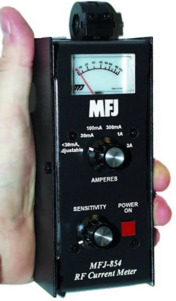
Above is the MFJ-854. It is a calibrated clamp RF ammeter. The manual does not describe or even mention its application for measuring common mode current.

So, my correspondent had measured the current in each wire of a two wire transmission line, recording 1.50 and 1.51A. He formed the view that since the currents were almost equal, the line was well balanced.

I have not used one of these, I rely on my correspondents guided measurements. (I have used the instrument described at Measuring common mode current extensively.)

MFJ-835

This is the instrument that MFJ sell for showing transmission line balance. One often sees recommendations by owners on social media, it is quite popular.

 

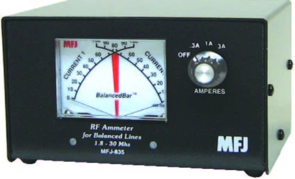
If the needles cross within the vertical BalancedBarTM the balance is within 10%. If not, you know which line is unbalanced and by how much.

Note the quote uses current like it is a DC current, not an AC current with magnitude and phase.

So, in the scenario mentioned earlier, the needles would deflect to 50% and 50.3% on the 3A scale, the needles would cross right in the middle of the BalancedBarTM, excellent.

… or is it?

One more measurement with the MFJ-854

I asked the chap to not only measure the (magnitude) of the current in each wire, but to pinch the wires together and close the clamp around both and measure the current. The remeasured currents were of 1.50 and 1.51A in each of the two wires, the current in both wires bundled together was 1.2A.

What does this mean?

With a bit of high school maths using the Law of Cosines, we can resolve the three measured currents into common mode and differential mode components.

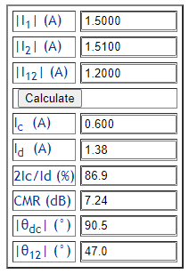
Above is the result, the current in each wire comprises a differential component of 1.38A and a common mode component of 0.6A. The common mode components in each wire are additive, so the total common mode current on the feed line is 1.2A.

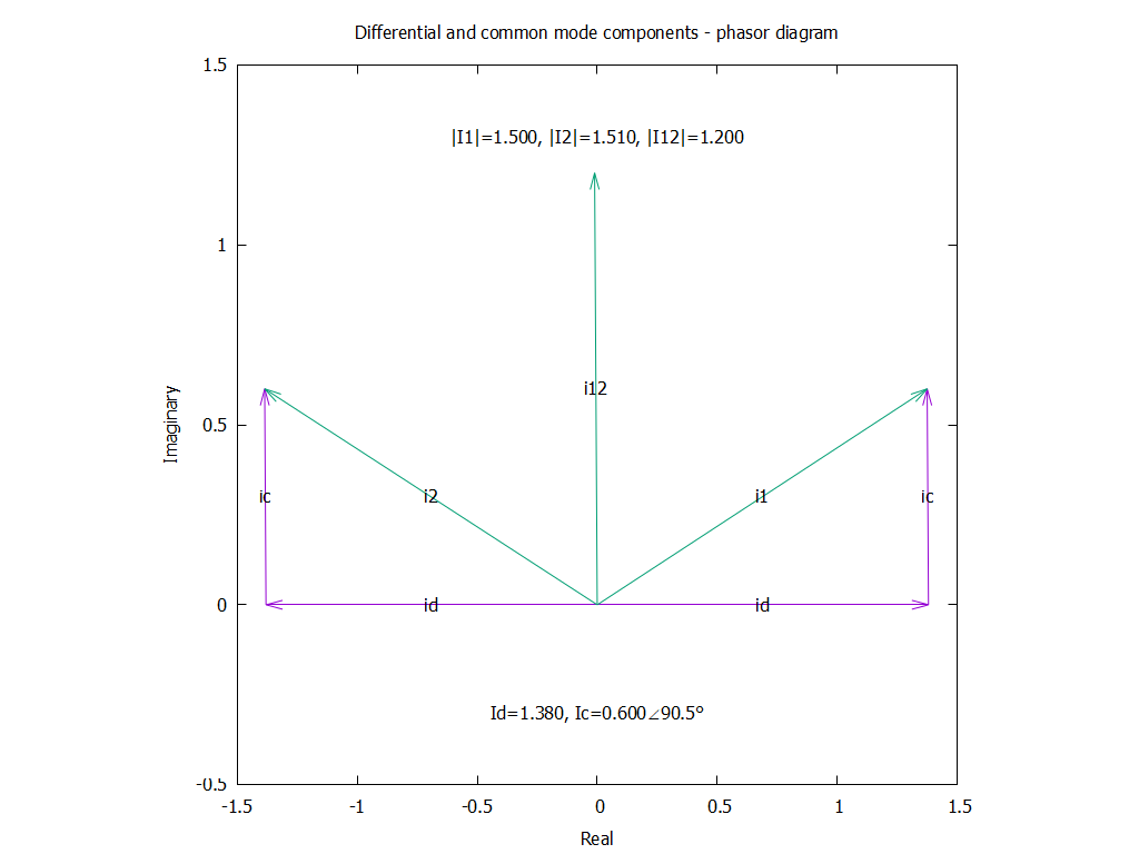
Above is a phasor diagram of I1, I2 and I12, and the components Ic and Id.

Note in this diagram that whilst the magnitude of i1 and i2 are similar, they are not 180° out of phase and that gives rise to the relatively large sum I12 (the total common mode component of I1 and I2).

This is a severe imbalance, sufficient to indicate a significant problem and to prompt a physical and electrical check of the antenna and feed line conductors and insulators.

Repairs were made and the measured result was quite good.

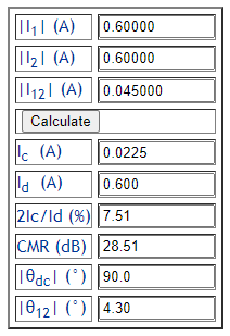
Above are the measurements and calcs.

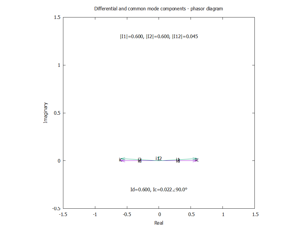
Above is the phasor diagram… a bit harder to read as there is very little common mode current.

By contrast with the previous case I1 and I2 are almost 180° out of phase and the sum of them, I12 has very small magnitude.

Conclusions

The MFJ-854 can be used effectively for measuring current balance.

Understanding the relative common mode and differential components hinted there was something very wrong in the antenna system.

Forget the MFJ-835 for proving balance. If the needles do not cross in the BalancedBarTM it indicates unbalanced amplitudes. If they do cross in the BalancedBarTM it indicates approximately balanced amplitude, but does not prove the phase relationship is approximately opposite and as shown in this example, is a quite erroneous result.

This article is a remeasure of NanoVNA-H4 – a ferrite cored test inductor impedance measurement – s11 reflection vs s21 series vs s21 pi using a VNWA-3E of both a good and sub-optimal test fixture estimating common mode choke impedance by three different measurement techniques:

• s11 shunt (or reflection);
• s21 series through
• s21 series pi;

Citing numerous HP (and successor) references, hams tend to favor the more complicated s21 series techniques even though the instruments they are using may be subject to uncorrected Port 1 and Port 2 mismatch errors. “If it is more complicated, it just has to be better!”

s21 series pi is popularly know as the “y21 method” (The Y21 Method of Measuring Common-Mode Impedance), but series pi better describes the assumed DUT topology.

What is an inductor?

Above is the test inductor, enamelled wire on an acrylic tube, an air cored solenoid.

We speak naively of this sort of component as an inductor, perhaps thinking it is a frequency independent inductance with perhaps some small series resistance. Let me make the distinction, Inductance is a property, Inductor is a practical thing (that includes Inductance… that might be a function of some variables).

Above is an s11 reflection measurement of the impedance of the air cored solenoid.

Above, focusing below about 5MHz, R is very low and X is approximately proportional to frequency, and the calculated equivalent series L is approximately independent of frequency… so the naive model discussed earlier might be adequate. Measured inductance at 1kHz is 20µH, at 5MHz apparent series inductance is still close to 20µH, but then starts rising, more quickly as the first resonance is approached (see previous plot).

We can calculate a value of shunt C that will resonate the inductor at this first resonance, in this case it is 1.02pF (often referred to as Cse). The parallel combination of 20µH and 1.02pF will have an impedance that is a good approximation of what was measured up to perhaps 1.2 times the frequency of the first resonance, BUT NOT ABOVE THAT. Such an equivalent circuit is useful, be be mindful of the acceptable frequency range.

The existence of higher order resonances shows that this is not simply an inductance. Calculated Cse will not explain the impedance curve much above the first resonance, it will NOT explain higher order resonances.

Understand the nature of the DUT

The DUT is a small test inductor, 6t on a Fair-rite 2843000202 binocular core (BN43-202).

We speak naively of this sort of component as an inductor, perhaps thinking it is a frequency independent inductance with perhaps some small series resistance.

You might look up the Al parameter for the core and calculate its inductance to be \(L=A_l n^2=2200*36=79,200 \text{ nH}\) and calculate its impedance @ 10MHz \(Z=\jmath 2 \pi f L=\jmath 2 \pi \text{ 1e7} \text{ 79.2e-6}=\jmath 4976\).

In fact it measures 3206+j1904, so the notion of a fixed inductance with small series resistance is not an adequate model for this component at HF. It exibits a first resonance at about 16.3MhHz.

In fact the DUT is a resonator, plotted here around its first resonance.

Using a ferrite core that is both lossy and frequency dependent permeability might make higher order resonances harder to observe, they are not simply harmonically related and they may be severely damped.

The test fixture

The test uses a small test inductor, 6t on a Fair-rite 2843000202 binocular core (BN43-202) and a small test board, everything designed to minimise parasitics. This inductor has quite similar common mode impedance to a HF good antenna common mode chokes.

Above is the SDR-KITS VNWA testboard.

The nanoVNA-H4 v4.3 was calibrated using the test board and its associated OSL components. The calibration / correction corrects Port 1 and Port 2 mismatch error. The test board is used without any additional attenuators, it is directly connected to the nanoVNA-H using 300mm RG400 fly leads.

Above, the test inductor mounted in the s11 shunt measurement position.

Above is the sub-optimal test setup, the DUT is connected by the green and white wires, each 100mm long.

Measurements and interpretation

Optimal

Above are the results of the three impedance measurement techniques.

Note that s21 series through and s21 series pi show no significant difference.

There is a difference between the s11 shunt method and the s21 series methods, the self resonant frequency is slightly different.

Sub-optimal

It is often held that the series pi or Y21 method corrects a sub-optimal fixture, but if you look closely, the series through and series pi curves have no significant difference between them, and they are only a little different to the plots from the optimal fixture… probably insignificant difference.

Does that mean series through undoes untidy fixtures in general? I doubt it.

Why the difference?

There are differences between the measurement methods, well between s11 shunt and s21 series through though in this case no significant difference from s21 series through to s21 series pi; and differences between the test jigs.

Note the test jig affected one measurement method differently to the other.

The results are sensitive to small changes in fixture layout, temperature, component tolerances etc

Sensitivity to parasitic fixture capacitance

Above is a chart of the measured s11 shunt impedance and two calculated values with 0.2pF of shunt capacitance subtracted and added. Note the effect on maximum R, and the self resonant frequency (SRF) (where X passes through zero).

From this information, we can calculate that the inductor at resonance is represented by some inductance with some series resistance, and Cse=1.5pF. So it is very easy for untidy fixtures, long connections etc to disturb the thing being measured.

BTW, for this DUT that is high impedance around resonance, 6mm of 200Ω transmission line (connecting wires?) has an equivalent Cse if about 0.2pF.

A rule to consider

A good measurement technician challenges his measurements, the fixtures, the instrument etc.

A guide I often give people is this:

if you reduce the length of connections and measure a significant difference, then:

• they were too long; and
• they may still be too long.

Iterate until you cannot measure a significant difference.

A challenge to your knowledge

Q: what is the formula for the resonant frequency of a parallel resonant circuit?

What you answer simply \(f=\frac1{2 \pi \sqrt{L C}}\) ?

Practical inductors also have an equivalent series R, and that is not included above… so it is a formula for ideal components, not for the real world.

A: that is the correct formula for a series resonant circuit, no matter how much series R is involved, and it is a good approximation for parallel resonant circuits with high Q, but has significant error for slow Q values (eg single digit.)

Why do I mention this?

Well, ferrite cored inductors may well have Q in the single digit domain, particularly broadband common mode chokes in the region of their SRF.

NanoVNA-App has been changed to improve the accuracy of s21 measurement.

The change is to implement Enhanced Response Correction.

NanoVNA-App-Setup-v1.1.209-OD18.exe

 

A correspondent asked my thoughts on a Youtube video featuring…

NE6F’s common mode current tester

Above is the schematic of NE6F’s common mode current tester.

The concept is that current probes A and B are placed either side of a current mode choke, and by calibrating and switching between them, a relative reading of current on one side compared to the other may be found.

Note that the two transformers are intended to be current transformers, they have a ratio of 1:10 turns so the \(Is=\frac{I_p}{n^2}=\frac{I_p}{100}\) … provided there is a low impedance load (called a burden) connected to the secondary.

If the burden was say 100Ω, then the current transformer inserts an impedance of approximately 100/10^2=1Ω in the primary circuit. If a current sensing element does not have a very low impedance, it is likely to disturb the thing being measured.

A general rule about current transformers is that if there is no burden on a current transformer:

• excessive / dangerous voltage may be developed by the secondary winding;
• a high impedance may be inserted in series with the primary line.

So, this is a current transformer with a burden of megohms, a deeply flawed design, but that problem is easily fixed by connecting a resistance of say 100Ω across each secondary winding.

Common mode current adjacent to a small choke

Consider a straight section of coaxial feedline not close to other materials, and with a small common mode choke inserted in the feedline. A “small” choke means one that is a very tiny fraction of a wavelength, say λ/100, from connector to connector.

Ask yourself that if say 1A of common mode current flows into one connector, what is the common mode current at the other connector?

What is your answer if you were told the balun was specified to have a CMRR of 20dB?

Take your time… a follow up will be posted in a day or three.

The fashion for measuring HF broadband common mode chokes for antenna systems is to use the s21 series through measurement technique, the basis for which is specious as discussed elsewhere on this blog.

Let’s look at an example common mode choke, this time for suppression of ham transmitter ingress to a VDSL2 line.

The spectrum of interest is 1.8 to 10.2MHz, this is the overlap between VDSL2 spectrum and ham bands above 1MHz.

Somewhat arbitrarily, a design specification was drawn up for a prototype choke which would be tested for effectiveness. The draft specification was:

• use of standard modular telephone cable with RJ12 ends for compatibility with the standard VDSL2 line hardware;
• no significant effect on differential mode (assisted by the above); and
• |Zcm|>2000Ω from 1.8 to 10.2MHz.

A prototype ferrite cored choke was designed and fabricated.

Above is the measurement of |Zcm| of the choke. The pink area denotes the limits of the specification, the measured trace must lie above the pink are to comply.

So, the prototype choke complies with the draft specification.

We are not interested in the maximum value of |Zcm|, the draft specification is written in terms of minimum |Zcm| from 1.8 to 10.2MHz.

So, our measurement concern is not about the accuracy of the trace at 5000Ω, but whether its accuracy at up to 2000Ω is sufficient for the purpose at hand (keeping in mind the very considerable tolerance of ferrite cores).

The common obsession with measuring the maximum value of |Zcm| when the minimum value of |Zcm| in the intended operating range by be much less seems quite illogical.

Whilst this article discusses a common mode choke for a VDSL2 line, the issues are not significantly different to a choke for an antenna system and the design might be well suited to an antenna system application over the same frequency range by substituting coax for the modular cable.

Above is measurement of |Zcm| of an antenna common mode choke described in this blog. In this case measured |Zcm|>2000Ω from 2.3 to greater than 30MHz, I have no interest in the maximum value (which occurs at about 6MHz).

Of course a direct better measure is one of Icm with the balun deployed in the target antenna system.

If you are a buyer perusing graphs of |Zcm| (if you find them), don’t be seduced by maximum |Zcm| (which might not even be within a band of interest), focus on the minimum |Zcm| in bands of interest.

This article reports a simple but robust measurement of the ReturnLoss of a pair of UHF adapters from 1 to 501MHz.

Load selection

To measure ReturnLoss of the adapter set, it must be terminated with a quality load, one that has an ReturnLoss better than the expected measurement.

Two loads are considered:

• Port 2; and
• a reference load.

Port 2 load

Above is a measurement of Port 2 ReturnLoss. This load cannot be used to measure ReturnLoss of higher than 14dB at 500MHz to uncertainty less than 3dB, so it is not a suitable load for measurement of ReturnLoss of the adapter set.

Reference load

The best available reference load is a SMA load that measures DC resistance of 49.805Ω and so we might infer that it has a low frequency ReturnLoss of 54dB.

This load was used to calibrate the VNA.

Let’s say we will accept uncertainty in ReturnLoss measurement of ±3dB.

Above is calculation of the ReturnLoss that can be measured using the 54dB reference to uncertainty of ±3dB, the result is 43dB.

The load will be a little poorer at higher frequencies, but the VNA firmware does not provide for a more detailed model of the load (or other calibration parts).

Above is measurement of the adapter set terminated in the reference load detailed above.

At 500MHz, the adapter pair could not be used in a test fixture to measure ReturnLoss of more than 10dB to uncertainty of ±3dB. ReturnLoss=10dB with uncertainty of ±3dB is equivalent to a VSWR confidence interval of 1.59-2.36.

At 100MHz, the adapter pair could not be used in a test fixture to measure ReturnLoss of more than 24dB to uncertainty of ±3dB. ReturnLoss=24dB with uncertainty of ±3dB is equivalent to a VSWR confidence interval of 1.09-1.18.

What is going on?

 

Above is a Smith chart view of s11 which gives insight. Note that it is an arc from about chart centre at lowest frequency, clockwise as frequency increases.

Let’s zoom in on it for more detail and analysis.

 

Above is a zoomed in view. The trace is not quite a circular arc, but there is a strong underlying circular trend with centre of the arc somewhere around 40+j0Ω which hints that the imperfection can be approximated as a short section of 40Ω transmission line in this case.

A 50mm bulkhead adapter example

Above is a longer adapter, a 50mm bulkhead adapter commonly used in panels for wall penetrations etc.

Above is a ReturnLoss plot to 500MHz. Note the different scale to the earlier chart.

Above is a Smith chart view of s11 which gives insight.

See Study of suitability of UHF bulkhead adapter to a Diamond x50-A antenna system for a deeper analysis of this adapter.

There must a a thousand articles on the ‘net on why UHF series connectors are good or bad, this is another.

The example

The example for discussion is a Diamond X-50A 2m/70cm vertical antenna on about 11m of LDF4-50A feed line, N type connectors are used throughout.

At commissioning, a sweep looking into the feed line was made using an Rigexpert AA600 analyser and the results saved. The file used for this study is a sweep from 143-151MHz.

Above is the UHF series bulkhead adapter studied in the simulation. It is 50mm end to end, the simulation uses 60mm to account for the impedance discontinuity in the mating plugs. The adapter is modelled as 60mm of lossless 35Ω line with VF=0.7 (typical of UHF series adapters).

This type of adapter is quite often used for an access panel penetration at a building entry at lengths up to 200mm.

Analysis

So, knowing the impedance looking into the feed line which normally connects to an N type bulkhead adapter, let’s model the VSWR curve seen looking into the example UHF series adapter (assuming the cable terminated in a UHF series plug.

The UHF series bulkead adapter will transform impedance, altering VSWR(50), and the effect will depend greatly on the feedline length, ranging from a best case to a worst case. This SimNEC model has two parts, one for best case and one for worst case, and each adjusts the feedline length a little to explore the limits of effect.

Above is a chart of measured and simulated results.

The blue and black lines are the VSWR curves for the measured feedline impedance adjusted a little for the best and worst cases.

The red curve is a best case, it is for the case where the feed line is 410mm shorter so that the phase of the reflected wave is such that that of the adapter reduces the reflection amplitude maximally. VSWR @ 147MHz is about 1.17, quite less than the baseline 1.4.

The green curve is a best case, it is for the case where the feed line is 35.5mm longer so that the phase of the reflected wave is such that that of the adapter reinforces the reflection amplitude maximally. VSWR @ 147MHz is about 1.69, quite more than the baseline 1.4.

Conclusions

The analysis is specific to the scenario, and results cannot be simply extrapolated to other scenarios. Each use case demands its own analysis.

The adapter, even though only 7° electrical length, significantly effects observed VSWR, in this case the VSWR looking into the adapter would range from 1.17 to 1.69 with very small changes in the LDF4-50A feed line.

I would not use such an adapter at 147MHz even though the transceiver’s use of UHF jack might imply wider fitness for purpose, and that these antennas are commonly sold with UHF connectors.

Power standing wave null… more left readers with “homework” to create the Pfwd and Prev traces.

Remember that Pfwd and Prev are interpretations in the context of some Zref of V and I at a point, and that \(P=P_{fwd}-P_{rev}=V_{fwd}I_{fwd}-V_{rev}I_{rev}\) is valid ONLY if Zref is purely real.

So let’s plot Pfwd and Prev wrt:

• Nominal Ro (ie the real part of the nominal Zo of the RG58A/U at 10MHz);
• 50Ω; and
• 75Ω to demonstrate the effect of different contexts, ie Zref.

Above IndFwd50 and IndFwdRo are almost coincident (at 10MHz Nominal Ro is very close to 50Ω), as are IndRev50 and IndRevRo. IndFwd75 and IndRev75 are separated from the others. In all cases, the IndFwdxx-IndRevxx is equal to p.

Note that if Zref is close to the line Zo, the shape of Pfwd and Pref are essentially a logarithmic decay in the direction of wave travel with a small superimposed cyclic variation.

If Zref is quite different to line Zo, the exponential element still exists but with a much larger cyclic variation along the line.

Above is a model of load VSWR=10, and p, Pfwd and Prev wrt 50Ω, and there is still the exponential element and only a relatively small cycle variation.

So, from those we learn that if you were to insert a 50Ω directional wattmeter at various points along a nominal 50Ω line, even with high VSWR, there will be only a small cyclic variation with displacement  and the exponential decay will be more significant.

The cyan trace is the voltage along the line, and you may observe that the ratio of max to min near to load is almost 10, VSWR at the load is 10, but measuring the first peak brings a little line loss to bear. The solid magenta curve is 50 times the current (so that it is viewable under the right hand axis scaling).

So, under mismatch there may be a wide variation in voltage and current along the line, but that will not be so apparent on a directional wattmeter which responds to both current and voltage and is sensitive to their phase relationship.

A point for pondering

Noting that in this example there is a small standing wave (VSWR=2), and that whilst Matched Line Loss (MLL per meter is uniform along the line, loss under standing waves is not uniform along the line. So the popular graphs that give you (uniform) line loss under standing waves based on VSWR and MLL are unsound, they are an approximation based on usually unstated assumptions.

Downloads

The download below contains the original SimNEC model, and a revised one with the above calcs and traces added.

SWDisplacement.7z

Power standing wave null? discussed the “Power Standing Wave” concept unfolding on social media.

Already a correspondent has asked if the graphs given in Power standing wave null? can be replicated in SimNEC.

They can. The original Mathcad graphs were wrt displacement from the source along the line to the load, and the sign of displacement is -ve (consistent with the Telegraphers Equation). So, that requires a bit of manipulation in SimNEC, and because SimNEC does not allow us to sample a TL element at an arbitrary displacement, the following model uses two TL elements of overall length 30m, and by adjusting the length of each we can move the observation point (T1 input).

The calculations of lengths and power are visible in the popups.

In a passive system, real power (ie watts) must decrease monotonically from source to load. Online postings showing otherwise attest to the knowledge of AC fundamentals of the modeller / poster.

Why (T1.V*Conj(T1.I)).R ?

This relies on basic principles of Alternating Current. The power at a point excited by a sine wave is \(P=V I^*\) (meaning V times conjugate of I) where V and I are RMS values, it is a complex quantity comprising the real power (watts) and reactive power (VAr). We are interested in the real power, so we multiply V times conjugate of I at T1 input, and take the real component of it for real power.

Homework

Interested readers can construct the other plots.

Downloads

SWDisplacement.7z

A social media posting in a very long thread with a lot of wooly thinking recently contained this explanation:

If you locate your power meter anywhere along the feedline other than at a POWER standing wave null, you will get a reading that is higher than the amount of power being delivered to the load.

A “Power Standing Wave”… hmmm, that is new to me.

The ensuing discussion may discuss this notion, probably in terms of lossless lines.

(Duffy 2008) develops several plots of interesting quantities with a load of 5+j50Ω on a length of RG58A/U using the  Telegraphers Equation.

Above is a plot from (Duffy 2008) Above shows P(x) vs displacement x, -ve x is on the source side of the load, at 10MHz with a load of 50+j50Ω where the modelled Zo is 50.4-j0.7Ω. Note that loss under mismatch is not uniform, the slope of P(x) varies with x.

Is this W6YK’s “Power Standing Wave”? There are no nulls, and the minimum is at the load.

A question for the reader, is \(P=P_{fwd}-P_{rev}\) measured at a point x with a directional wattmeter calibrated for 50+j0Ω, or is it simply the power passing that point?

What about the forward and reflected power measures?

Above shows the case at 10MHz with a load of 50+j50Ω where the modelled Zo is 50.4-j0.7Ω. Note the indicated power levels for forward and reflected waves calculated based on a directional wattmeters calibrated to nominal Zo (Ro) and actual Zo.

Conclusions

So I am left wondering what “Power Standing Wave” means.

References:

Duffy, O. 04/2008. VSWR and displacement.

Directional wattmeters are used in lots of ham stations, yet we see evidence in social media posts that many people do not understand them and the measurement context.

We have an RF source connected via a Bird 43 directional wattmeter with an appropriate 50Ω measurement element directly to a load resistance.

We measure the load voltage to be 100Vrms and the current to be 1Arms.

1. What is the power in the load?

100W

2. What does the directional wattmeter indicate for Pfwd?

112.5W

3. What does the directional wattmeter indicate for Prev?

12.5W

What is the implied VSWR?

2

4. Can the load power in this scenario be ‘measured’ using this instrument?

Yes, since the calibration impedance is a purely real value, measure Pfwd and Pref and calculate P=Pfwd-Prev.

Any surprises there?

Explanations to follow in the coming days.

Recently on QRZ, KL7AJ opened a thread recommending his own slide presentation entitled “SWR meters make you stupid”.

After more than 100 posts, one of the participants tried to understand this diagram for the presentation.

Now there may have been some discussion at the meeting where this was presented, giving details that are missing from the slides.

Lets assume that all transmission lines are 50Ω lossless line, and that the calibration of the wattmeters is wrt 50+j0Ω.

If we start with a literal interpretation of what is presented, starting at the load which determines the VSWR seen by wattmeter #2 in this case, since VSWR=4 we can calculate rho=0.6, rho^2=0.36 and that Pfwd is Prfl/rho^2=36/0.36=100W.

Now we have Pfwd and Prfl, we can calculate P=Pfwd-Prfl=100-36=64W.

Looking at wattmeter #1, P=Pfwd-Prfl=100-0=100W.

So, there is 100W into the TUNER and 64W out, it has a loss of 1.9dB.

That is not an extraordinary loss for a TUNER, it is not so ridiculous as to be an obvious mistake… but it may not be what the author had in mind.

It is also possible that the stated Prfl=36W at wattmeter #2 was a mistake? An exercise for the reader is to calculate Prfl and Pfwd at wattmeter #2 if the TUNER was lossless, is it a problem that Pfwd is greater than the transmitter output power?

Directional wattmeters are used in lots of ham stations, yet we see evidence in social media posts that many people do not understand them and the measurement context.

We have an RF source connected via a Bird 43 directional wattmeter with an appropriate 50Ω measurement element directly to a load resistance.

We measure the load voltage to be 100Vrms and the current to be 1Arms.

1. What is the power in the load?
2. What does the directional wattmeter indicate for Pfwd?
3. What does the directional wattmeter indicate for Prev?
4. What is the implied VSWR?
5. Can the load power in this scenario be ‘measured’ using this instrument?

Get your slide rules out, jot your answers down. My answers in a day or two…

Recently on social media, F6AWN cited a “document written by a team of engineers working in a company of 12,000 people devoting to perfecting power” which ended with the following formula:

The paper does not state that the phasors are RMS, RMS phasors, but it appears so… so let’s use like.

Taking the expression \(P_{load}=\frac{|V_f|^2}{Z_0}-\frac{|V_r|^2}{Z_0}\), on the surface of it, it appears to be subtracting one power quantity from another, \(P=P_f-P_r\). Electric field components can be superposed, so can magnetic field components, and in a transmission line, the equivalent voltages and currents can be superposed, but powers cannot be superposed (read up on the Superposition Principle).

So the original quoted formulas do not apply as generally as written.

That said, we often loosely say \(P=P_f-P_r\), but is it always true, sometimes true, never true?

Well, the answer is that it is sometimes true, it is true when Zo is purely real, see Power in a mismatched transmission line.

There are two cases where Zo is sufficiently close to purely real that the error in applying \(P=P_f-P_r\) is small to insignificant:

1. using practical transmission lines at a frequency high enough that Zo is approximately real; and
2. measurements with a sampler that transforms a point sample of voltage and current into Pf and Pr for some real calibration impedance.

An example of the latter would be use of a properly calibrated Bird 43 with 50Ω element which is calibrated for Zref=50+j0Ω. Note that if you insert such an instrument into a line with actual Zo=50-j1, whilst the displayed value of Pf and Pr of themselves are slightly in error, calculated \(P=P_f-P_r\) is correct (see Power in a mismatched transmission line which BTW uses amplitude of phasors rather than RMS.)

This brings us to related bit of traditional ham wisdom posted recently on social media, Warren Allgyer stated:

Power readings on 50 ohm instruments like a Bird 43, and SWR meter, or even the output power meter of a transceiver are not accurate unless made at a 50 ohm point.

The only specific instrument mentioned is a Bird 43 (Directional Wattmeter), the other two are non-descript, more later.

In respect of the Bird 43, as explained earlier, the Bird 43 samples V and I in a very small region, approximately at a point, and transforms a point sample of voltage and current into Pf and Pr for some real calibration impedance, usually 50+j0Ω. As explained above, calculated \(P=P_f-P_r\) is correct, even if Zo departs from 50+j0Ω, even if Zo=75-j2Ω. Whilst the net power calculated is correct, the stand alone values of Pf and Pr are only exactly correct wrt 50+j0Ω and VSWR calculated from them is VSWR that would exist on a line of Zo=50+j0Ω.

If you were to use such an instrument in a line where Pr is not equal to zero, whilst Pf and Pr do not have stand alone value, the quantity \(P=P_f-P_r\) is correct, you can measure the ‘net’ power in a line even in the presence of standing waves. The traditional ham wisdom quoted above is wrong.

The only comment that can be made about “SWR meter, or even the output power meter of a transceiver” is that if they transform a point sample of voltage and current into Pf and Pr for some real calibration impedance, usually 50+j0Ω, they behave as explained for the Bird 43. Just because a transceiver incorporates a directional coupler to measure VSWR for display and protection circuits, it does not mean its power meter displays Pf.

Now polite people on social media do not call out errors like these, so they remain unchallenged for the gullible to learn and recite later themselves.