Ian White gives the following diagram to explain what goes on at the coax to dipole junction.

He labels five currents in his explanation.

Let’s simplify that

Above is a diagram from Common mode current and coaxial feed lines showing the currents where a coax connects two two wires.

Lets morph that to the dipole feedpoint topology.

The whole thing is defined by just two currents, I1 and I2. The common mode current Ic=I1-I2. There is common mode current present in the short two wire connection to the dipole, and on the outer surface of the coaxial cable.

Note that I1, I2 and Ic are usually standing waves (ie they vary with location), and so these currents are defined here at the point where the conductors meet the end of the coax.

Are the currents measurable?

Using a clamp on RF current probe, the currents on the each of the two dipole conductors I1 and I2 is measurable, and so also the current on the outside surface of the coax shield Ic.

Remember also that these are sinusoidal AC currents, and I1, I2 and Ic refer to the magnitude of the currents.

The three currents can be resolved into the common mode and differential components, see Resolve measurement of I1, I2 and I12 into Ic and Id
(I12=Ic, the current measured with the probe around both two wire conductors or around the outside of the coax.

Can the currents be measured at an elevated dipole feed point?

Sure. I have done measurements of Ic over the length of coax by hoisting a current probe on a separate halyard to raise and lower it and reading it from the ground with a spotting scope.

Recall that Ic is usually a standing wave, and when you measure it at just one point, you don’t know much about it.

I see online discussion of specification bending radius for coax cables, and their application to ferrite cored common mode chokes.

A low Insertion VSWR high Zcm Guanella 1:1 balun for HF and follow on articles described a balun with focus on InsertionLoss.

Let’s remind ourselves of the internal layout of the uncompensated balun.

The coax is quality RG58A/U with solid polythene dielectric. The coax is wound with a bending radius of about 10mm, way less than Belden’s specified minimum bending radius of 50mm.

So, the question is does this cause significant centre conductor migration that will ruin the characteristic impedance:

• when it was first constructed; and
• through life.

Note the pigtails at each coax connector, they are a departure from Zo of the coax and the N type connectors. They can be seen as short sections of transmission line with Zo perhaps 200Ω or more. The effect of these is to transform impedance and so cause the input VSWR to depart from ideal.

When first constructed

Above is a chart from the original construction articles. InsertionVSWR @ 30MHz is about 1.15.

Note the pigtails at each coax connector, they are a departure from Zo of the coax and connectors. They can be seen as short sections of transmission line with Zo perhaps 200Ω or more. The effect of these is to transform impedance and so cause the input VSWR to depart from ideal.

After 5 years of service

This article presents measurement of the balun 5 years after it was made, 5 years in use, but not operated at temperatures above datasheet maximum.

As mentioned, the pigtails are the main contribution to InsertionVSWR. The balun was compensated using 10pF shunt capacitors at both coax connectors. (Possible compensation solutions were discussed at A low Insertion VSWR high Zcm Guanella 1:1 balun for HF – more detail #3).

Above is a NanoVNA screenshot of measurement of the compensated balun using the calibration LOAD, a couple of SMA(F)-N(M) adapters and a short SMA(M)-SMA(M) cable.

InsertionVSWR is highest at 1.01 @ 16MHz, at the limits of accuracy with this equipment. These 3kV 10pF ceramic capacitors have measured Q around 500 at 30MHz, expected loss is less than 200mW @ 1kW through.

The InsertionVSWR is not significantly affected by the quite small bending radius.

Voltage withstand

Does tight bending of this cable degrade voltage withstand of the balun?

Experience Hipot testing lots of baluns with this type of coax winding shows that the voltage withstand weakness is over the surface of the dielectric from braid to centre conductor, and pigtails of less than 15mm will flash over before internal flashover.

Alternative coax types

Coax with a solid PTFE dielectric is more suitable as the dielectric is harder and withstands higher temperatures before deformation.

Foamed dielectric cables are much more prone to migration of the centre conductor on tight bends, even at room temperature and are probably unsuitable for tight wraps.

Small diameter cables might seem the obvious answer, but they are higher in loss and will run at higher temperature.

Conclusions

Though the coax bend radius is substantially smaller than specification minimum bend radius:

• when first constructed, there was little evidence that the coax characteristic impedance was altered by the winding radius, and that the pigtails were the main contribution to InsertionVSWR; and
• after five years of service, the InsertionVSWR of the compensated balun is excellent, at the limits of accuracy of the test equipment and again, little evidence that the coax characteristic impedance was altered by the winding radius.

Solid dielectric coax may be quite satisfactory at static tight bend radius, subject to the temperature of operation and applied forces.

Background

From time to time, ham radio operators may question whether a section of installed and used coax is still good or significantly below spec and needs replacement.

A very common defect in coax installed outside is ingress of water. The earliest symptoms of water ingress are the result of corrosion of braid and possibly centre conductor, increasing conductor loss and therefore matched line loss (MLL). Any test for this must expose increased MLL to be effective.

Introduction

This article describes a simple but effective test of MLL for coax of known Z0 and length using a suitable one port antenna analyser (or VNA such as the NanoVNA), the nominal Z0 is sufficient to demonstrate cable is good.

The test involves measuring the resistance looking into a resonant length of coax with either an open circuit or short circuit termination.

The concept is to measure MLL and compare it to specification. Defects that increase MLL are not usually narrowband, but will be evidenced over a very wide range of frequencies so measurement at the exact operating frequency is not necessary.

Analyser requirements

Frequency

The analyser will need to cover a suitable frequency range for measurement. For cables for use on HF, I would advise measurement above 10MHz as actual Z0 is closer to nominal Z0. For higher frequencies, choose a range near to the operating frequency.

The analyser needs to be able to measure R and X reasonably accurately at a low impedance or high impedance resonance of the line section with either SC or OC termination.

Access

Access is needed to one end for the analyser, and at the other end for a SC or OC termination (the cable has to be disconnected from the antenna). It is not necessary to connect the ‘far end’ back to the analyser as you would for a two port transmission test.

Connectors

If you use connectors with a loose coupling sleeve (UHF, SMA etc), do not use a loose male connector as OC, connect it to a F-F adapter so nothing is loose.

To get accurate results, all connectors must be secure, clean and properly tightened.

Got all that under control? Let’s measure…

A practical example

The DUT is 10m of quite old budget RG58A/U fitted with crimp BNC connectors. A sample of this cable has previously been measured for braid coverage, it is just 78% so we might expect it to be a little poorer than Belden 8259.

Above, the top is a sample of the cable under test, and lower is Belden 8259. One can see the poorer braid coverage of the test cable… but does that alone condemn it?

The analyser is an AA-600 which uses an N(F) connector so a N(M)-BNC(F) adapter is used. The AA-600 uses a 16bit ADC, so it gives very good accuracy of extreme impedances (which is the case for this test).

Taking my own advice to measure above 10MHz, the third low impedance resonance of the cable section with OC termination is about 15MHz… let’s measure that.

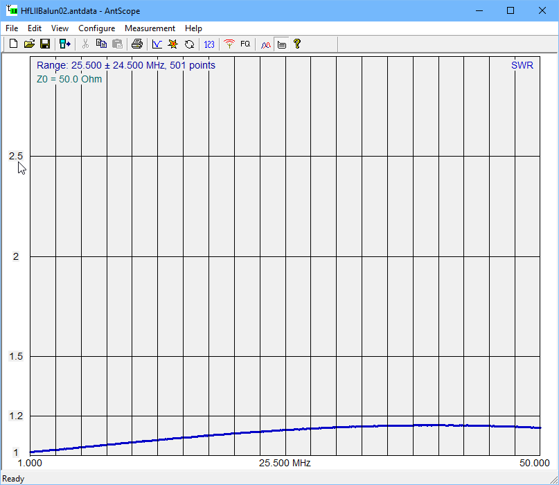
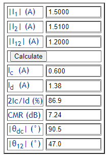
Using the AA-600’s measure All facility and scrolling frequency up and down with the arrow keys until X passes through zero, we get the above measurements. I have taken a screen shot for the article, but no USB connection is needed for a practical measurement, just write down the frequency and R when X=0.

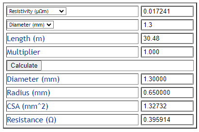
Now using Calculate transmission line Matched Line Loss from Rin of o/c or s/c resonant section we will calculate MLL (see Measuring matched line loss).

So, now we know the frequency of measurement and MLL, we need to find the specification MLL at that frequency using a GOOD line loss calculator.

Specification MLL is 0.06dB/m, we measured 0.07dB/m, it is a little higher than spec, probably a result of the budget construction, and no reason to condemn it, it is probably as good as the day it was made.

Can you use a NanoVNA?

Yes, you can any instrument that can measure R and X at resonance. I have demonstrated the technique using a noise bridge, an antenna impedance bridge (GR1606B), and a NanoVNA.

Conclusions

The technique and formulas used gives a practical simple but effective method of measuring matched line loss using a one port analyser (or any instrument that can measure R and X at resonance).

I have found you can never have enough of these things. It is very convenient to leave some measurement projects set up while work continues on some parallel projects.

Above is the kit as supplied (~$8 on Aliexpress). Note that it does not contain any male turned pin header… more on that later.

I was critical of Alixpress four years ago when I purchased the last one, but things have improved greatly in that time, to the point they are often faster delivery that eBay’s “Australian stock” sellers.

Carefully break off 7 x 7 way pieces of the turned pin female header and ‘dry’ fit them to the board, Now get two more pieces of header that are at least 7 way, and plug them at right angles to the ones already placed to set the spacing. Now solder them to the board (hint: liquid flux makes this job easier.) The ‘donuts’ are quite small, use a tip that gives contact to the donut so that heat is applied to the pin and the ‘tube’ for a good solder joint.

Test the coax connectors on a good male connector to be sure they are not defective… quality of these is poor. I tighten them to 0.8Nm to seat and form the female connector. If the threads bind, chuck them now rather than after you have soldered them in place.

I installed only the mid connectors on this board, I have another which has all the connectors and I have never used the other four. Carefully position and solder the connectors, again liquid flux helps.

The clear plinth does not come in the kit, it is my addition.

Above, the plinths designed in Freecad were cut out of 3mm clear PVC.

They are cut using a single flute 2mm carbide cutter.

You could easily make them with hand tools and a drill. M2.5×6 nylon screws are used to attach the plinth to the hex spacers (supplied), giving the assembly four non-scratch feet.

Now the kit is incomplete. You are going to need some parts you see above built on male turned pin header strip. The kit does contain some 49.9Ω resistors you can use for a LOAD, you will also need an OPEN (centre left) and a SHORT (lower right). Others are for connecting the sections of the test board and THROUGH calibration.

The SMA connector at left is another test fixture which uses the same calibration parts. It can be used directly on the NanoVNA or at the end of a convenient length of cable. I originally made it to use on a Rigexpert AA600, either on a N(M)-SMA(F) adapter, or a short N(M)-SMA(F) cable.

It is bit hard to see the connections on the board when it is populated, so I have made the graphic above, printed it and laminated it for handy reference.

Note that the connections are a little different to the SDR-Kits jig (that they probably copied), in particular C2, C6, E2 and E6 are each not connected to anything.

I have some custom made 300mm long RG400 cables that I use with these, labelled for calibration purposes. IIRC they cost about $30 per pair from RFSupplier.com.

Dave Casler sets out in his Youtube video to answer why two wire transmission line has so little loss . With more than 10,000 views, 705 likes, it is popular, it must be correct… or is it?

He sets a bunch of limits to his analysis, excluding frequency and using lossless impedance transformation so that the system loss is entirely transmission line conductor loss.

He specified 300Ω characteristic impedance using 1.3mm copper and calculates the loop resistance, the only loss element he considers, to be 0.8Ω.

Above is Dave’s calculation. Using his figures, calculated \(Loss=\frac{P_{in}}{P_{out}}=\frac{100}{100-0.27}=1.0027\) or 0.012dB.

Above is my calculation of the DC resistance at 0.395Ω per side, so I quite agree with his 0.8Ω loop resistance… BUT it is the DC resistance, and the RF resistance will be significantly higher (skin effect and proximity effect).

Casler’s is a DC explanation.

Self taught mathematician Oliver Heaviside showed us how to calculate the loss in such a line.

Let’s calculate the loss for that scenario more correctly.

Above is the complete output from RF Two Wire Transmission Line Loss Calculator.

One of the results shows the values of distributed R, L, G and C per meter, and R is 0.486Ω/m or 14.81 for the 30.48m length, nearly 20 times Dave Casler’s 0.8Ω.

Unsurprisingly, the matched line loss is larger, calculated at 0.213dB, much higher than Dave Casler’s 0.12dB.

Now for a bunch of reasons, the scenario is unrealistic, but mainly:

• the conductor diameter is rather small, smaller than many 300Ω commercial lines and impractical for a DIY line; and
• two wire line is most commonly used with high standing wave ratio and the often ignored loss under the specific mismatch scenario is more relevant.

Conclusion

It is common that the loss in two wire line system underestimates the line loss under mismatch and impedance transformation that may be required as part of an antenna system.

Casler’s DC explanation appeals to lots of viewers, probably hams, and might indicate their competence in matters AC, much less RF.

… Read widely, question everything!

This article reports and analyses a user experiment measuring current in a problem antenna system two wire transmission line.

A common objective with two wire RF transmission lines is current balance, which means at any point along the transmission line, the current in one wire is exactly equal in magnitude and opposite in phase of that in the other wire.

Note that common mode current on feed lines is almost always a standing wave, and differential mode current on two wire feed lines is often a standing wave. Measurements at a single point might not give a complete picture, especially if taken near a minimum for either component.

MFJ-854

The correspondent had measured feed line currents using a MFJ-854.

Above is the MFJ-854. It is a calibrated clamp RF ammeter. The manual does not describe or even mention its application for measuring common mode current.

So, my correspondent had measured the current in each wire of a two wire transmission line, recording 1.50 and 1.51A. He formed the view that since the currents were almost equal, the line was well balanced.

I have not used one of these, I rely on my correspondents guided measurements. (I have used the instrument described at Measuring common mode current extensively.)

MFJ-835

This is the instrument that MFJ sell for showing transmission line balance. One often sees recommendations by owners on social media, it is quite popular.

If the needles cross within the vertical BalancedBarTM the balance is within 10%. If not, you know which line is unbalanced and by how much.

Note the quote uses current like it is a DC current, not an AC current with magnitude and phase.

So, in the scenario mentioned earlier, the needles would deflect to 50% and 50.3% on the 3A scale, the needles would cross right in the middle of the BalancedBarTM, excellent.

… or is it?

One more measurement with the MFJ-854

I asked the chap to not only measure the (magnitude) of the current in each wire, but to pinch the wires together and close the clamp around both and measure the current. The remeasured currents were of 1.50 and 1.51A in each of the two wires, the current in both wires bundled together was 1.2A.

What does this mean?

With a bit of high school maths using the Law of Cosines, we can resolve the three measured currents into common mode and differential mode components.

Above is the result, the current in each wire comprises a differential component of 1.38A and a common mode component of 0.6A. The common mode components in each wire are additive, so the total common mode current on the feed line is 1.2A.

Above is a phasor diagram of I1, I2 and I12, and the components Ic and Id.

Note in this diagram that whilst the magnitude of i1 and i2 are similar, they are not 180° out of phase and that gives rise to the relatively large sum I12 (the total common mode component of I1 and I2).

This is a severe imbalance, sufficient to indicate a significant problem and to prompt a physical and electrical check of the antenna and feed line conductors and insulators.

Repairs were made and the measured result was quite good.

Above are the measurements and calcs.

Above is the phasor diagram… a bit harder to read as there is very little common mode current.

By contrast with the previous case I1 and I2 are almost 180° out of phase and the sum of them, I12 has very small magnitude.

Conclusions

The MFJ-854 can be used effectively for measuring current balance.

Understanding the relative common mode and differential components hinted there was something very wrong in the antenna system.

Forget the MFJ-835 for proving balance. If the needles do not cross in the BalancedBarTM it indicates unbalanced amplitudes. If they do cross in the BalancedBarTM it indicates approximately balanced amplitude, but does not prove the phase relationship is approximately opposite and as shown in this example, is a quite erroneous result.