Ian White gives the following diagram to explain what goes on at the coax to dipole junction.

He labels five currents in his explanation.

Let’s simplify that

Above is a diagram from Common mode current and coaxial feed lines showing the currents where a coax connects two two wires.

Lets morph that to the dipole feedpoint topology.

The whole thing is defined by just two currents, I1 and I2. The common mode current Ic=I1-I2. There is common mode current present in the short two wire connection to the dipole, and on the outer surface of the coaxial cable.

Note that I1, I2 and Ic are usually standing waves (ie they vary with location), and so these currents are defined here at the point where the conductors meet the end of the coax.

Are the currents measurable?

Using a clamp on RF current probe, the currents on the each of the two dipole conductors I1 and I2 is measurable, and so also the current on the outside surface of the coax shield Ic.

Remember also that these are sinusoidal AC currents, and I1, I2 and Ic refer to the magnitude of the currents.

The three currents can be resolved into the common mode and differential components, see Resolve measurement of I1, I2 and I12 into Ic and Id
(I12=Ic, the current measured with the probe around both two wire conductors or around the outside of the coax.

Can the currents be measured at an elevated dipole feed point?

Sure. I have done measurements of Ic over the length of coax by hoisting a current probe on a separate halyard to raise and lower it and reading it from the ground with a spotting scope.

Recall that Ic is usually a standing wave, and when you measure it at just one point, you don’t know much about it.

An example of the utter nonsense posted on social media.

My very first posting as a trainee was to Bringelly HF receiving station in 1970. It had Rhombic antennas every 30° of the compass, and a few other antennas, but the mainstay of operation was the set of Rhombics.

The nearby transmitting station at Doonside had a similar antenna arrangement of Rhombics fed with two or four wire open transmission lines to transmitters in a central building, for most operations, no coax involved between transmitters up to 30kW and antenna feed points.

Rhombics are an example of a non-resonant antenna, these were used for a large set of operating frequencies that were not harmonically related, were changed through the day with varying ionospheric conditions over the various circuits, within the broad frequency range of the Rhombics, and not restricted by a requirement for ‘resonant length’ of radiator conductors.

You do not have to look hard for other examples of non-resonant length radiators that have good radiation efficiency.

Yet hammy Sammy thinks that ‘resonance’, whatever it means, is a necessary condition for radiation efficiency.

In this case, the quote speaks to the credibility of the author.

Social media and errors

A further disadvantage of lots of social media platforms is the inability to edit mistakes. For example, one poster wrote in the same thread:

The qualitative conclusion here is that a “wild” impedance value of 890 – j418 which is far from resonance can and does yield an acceptable SWR.

My calc is that wrt 50Ω, that example has VSWR=21.7. We all make mistakes, but this appears locked in for perpetuity.

And of course it is unsociable to call out factual error on social media.

So what happened to Bringelly and Doonside?

Bringelly part of the new western Sydney airport and Doonside is a major road interchange (the Light Horse Interchange).

I see online discussion of specification bending radius for coax cables, and their application to ferrite cored common mode chokes.

A low Insertion VSWR high Zcm Guanella 1:1 balun for HF and follow on articles described a balun with focus on InsertionLoss.

Let’s remind ourselves of the internal layout of the uncompensated balun.

The coax is quality RG58A/U with solid polythene dielectric. The coax is wound with a bending radius of about 10mm, way less than Belden’s specified minimum bending radius of 50mm.

So, the question is does this cause significant centre conductor migration that will ruin the characteristic impedance:

• when it was first constructed; and
• through life.

Note the pigtails at each coax connector, they are a departure from Zo of the coax and the N type connectors. They can be seen as short sections of transmission line with Zo perhaps 200Ω or more. The effect of these is to transform impedance and so cause the input VSWR to depart from ideal.

When first constructed

Above is a chart from the original construction articles. InsertionVSWR @ 30MHz is about 1.15.

Note the pigtails at each coax connector, they are a departure from Zo of the coax and connectors. They can be seen as short sections of transmission line with Zo perhaps 200Ω or more. The effect of these is to transform impedance and so cause the input VSWR to depart from ideal.

After 5 years of service

This article presents measurement of the balun 5 years after it was made, 5 years in use, but not operated at temperatures above datasheet maximum.

As mentioned, the pigtails are the main contribution to InsertionVSWR. The balun was compensated using 10pF shunt capacitors at both coax connectors. (Possible compensation solutions were discussed at A low Insertion VSWR high Zcm Guanella 1:1 balun for HF – more detail #3).

Above is a NanoVNA screenshot of measurement of the compensated balun using the calibration LOAD, a couple of SMA(F)-N(M) adapters and a short SMA(M)-SMA(M) cable.

InsertionVSWR is highest at 1.01 @ 16MHz, at the limits of accuracy with this equipment. These 3kV 10pF ceramic capacitors have measured Q around 500 at 30MHz, expected loss is less than 200mW @ 1kW through.

The InsertionVSWR is not significantly affected by the quite small bending radius.

Voltage withstand

Does tight bending of this cable degrade voltage withstand of the balun?

Experience Hipot testing lots of baluns with this type of coax winding shows that the voltage withstand weakness is over the surface of the dielectric from braid to centre conductor, and pigtails of less than 15mm will flash over before internal flashover.

Alternative coax types

Coax with a solid PTFE dielectric is more suitable as the dielectric is harder and withstands higher temperatures before deformation.

Foamed dielectric cables are much more prone to migration of the centre conductor on tight bends, even at room temperature and are probably unsuitable for tight wraps.

Small diameter cables might seem the obvious answer, but they are higher in loss and will run at higher temperature.

Conclusions

Though the coax bend radius is substantially smaller than specification minimum bend radius:

• when first constructed, there was little evidence that the coax characteristic impedance was altered by the winding radius, and that the pigtails were the main contribution to InsertionVSWR; and
• after five years of service, the InsertionVSWR of the compensated balun is excellent, at the limits of accuracy of the test equipment and again, little evidence that the coax characteristic impedance was altered by the winding radius.

Solid dielectric coax may be quite satisfactory at static tight bend radius, subject to the temperature of operation and applied forces.

This article is principally a short commendation for Jupyter or Interactive Python for ham radio related projects for the quantitative ham. Python is a cross platform programming language that has a very rich set of libraries to support scientific and engineering applications, and a good graph maker.

The exercise for this demonstration is to decompose three measurements of currents on a two wire transmission line at a point into the differential and common mode components at that point, and to plot a phasor diagram of a solution to the measurements. Remember that common mode current and differential current in an antenna system are usually standing waves.

Above is a diagram explaining the terms used, I1 and I2 are the magnitudes of currents in each conductor measured using a clamp on RF ammeter, and I12 is the magnitude of the current when both conductors are passed through the clamp on RF ammeter, i12 is the phasor sum of the underlying i1 and i2.

The solution to the problem lies in applying the Law of Cosines to find the angular relationship between the differential and common mode components, a high school trigonometry problem. In fact, we find the magnitude of the angle between ic and id.

Above is the solution, a phasor diagram taking id as the phase reference (ie 0°). Because we know only the magnitude of the angle between ic and id, there is a second possible solution as noted on the graphic.

Above is a screen capture of the Jupyter source cells and results.

When you look at the measurements that were taken, |i1| was within 2% of |i2| which many online experts would opine means there is nearly perfect balance. Measurement instruments based on simply comparing |i1| and |i2| indicating within the BalanceBar are deeply flawed… though very popular.

The decomposition shows that the magnitude of the differential current |id| is 25.7A and the magnitude of the total common mode current is 9.3A (4.65A per leg). It is not nearly balanced!

This demonstration uses high school mathematics applied to three measurements of current to drill down on the distribution of currents in a scenario that many would regard as balanced. Balanced means that the currents in each wire are equal but opposite in phase at any point along the line.

A quotation from Lord Kelvin:

When you can measure what you are speaking about, and express it in numbers, you know something about it. But when you cannot measure it, when you cannot express it in numbers, your knowledge is of a meagre and unsatisfactory kind. It may be the beginning of knowledge but you have scarcely in your thoughts advanced to the state of science.

One sees analyser sweeps of EFHW measurements posted online quite frequently, and a trend is that posters are quite pleased with the results.

Above is an example, a ‘user’s’ MyAntennas.com EFHW-4010 antenna with 23m of unspecified coax. Unfortunately it is a bit narrow, ordered up by an online expert.

The responses to the post were inevitably a focus on the location of the VSWR minima, and the value of VSWR at those locations.

But before focussing on the location of the resonances, I was taken with the rather compressed VSWR range. Let’s present that as ReturnLoss.

Above is ReturnLoss from the same .s1p file. For a shortish antenna, we might usually expect that the ReturnLoss minima will be quite a lot lower. Yes, these are out of band, but should not be dismissed as irrelevant.

Let’s look at an NEC model of a 21m long InvertedL EFHW.

Above is magnitude of Reflection Coefficient or ρ at the feedpoint (Zref=2450Ω) for a native EFHW as an Inverted L, ReturnLoss=-ρ (the chart is upside down compared to the previous one). Note that the ReturnLoss minima are up to about 1.2dB (recall that this model has no transformer loss, feed line loss, counterpoise on the ground loss).

The loss that results in high minimum ReturnLoss is likely to be a broaband loss, ie to affect in-band performance as well as between desired bands.

This begs the question, does the user’s antenna system contain some broadband loss mechanism that masks the natural impedance variation of the native EFHW?

If so, is there perhaps 2dB or more of broadband system loss that degrades RadiationEfficiency by as much as 40%.

Note also that there are fewer minima and maxima in the NEC model. The OP’s antenna with 5 distinct peaks shows signs of being electrically longer… the notion that the counterpoise is not part of the antenna length is wrong. So before focus on the location of ReturnLoss maximum (ie the ‘tuning’) there is an issue with the number of maxima and minima… this antenna is not working like a simple 40m EFHW on harmonics.

Since the widespread takeup of the NanoVNA, a measure of performance proposed by (Skelton 2010) has become very popular.

His measure, Common Mode Rejection Ratio (CMRR), is an adaptation of a measure used in other fields, he states that he thinks the application of it in the context of antenna systems and baluns is novel and that “CMRR should be the key figure of merit”.

Skelton talks of different ways to measure CMRR, but essentially CMRR is a measure of the magnitude of gain (|s21|) from Port 1 to Port 2 in common mode, with the common mode choke (or balun) in series from the inner pin of Port 1 to the inner pin of Port 2.

Note that this is the same connection as used for series through impedance measurement, but calculation of impedance depends on the complex value s21.

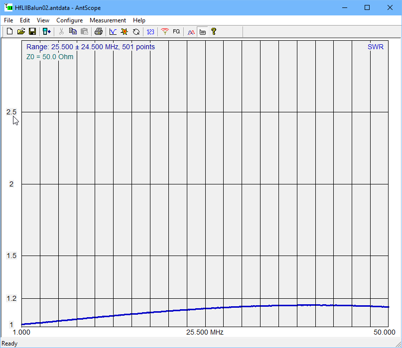
Above is capture of a measurement of a Guanella 1:1 common mode choke or balun. The red curve is |s21|, the blue and green curves are R and X components of the choke impedance Zcm calculated from s21.

Matched vs mismatched DUT

Case 1: impedance matched DUT

In this type of test, the DUT between Port 1 and Port 2 is a good match to both Port 1 and Port 2.

Lots of readers will understand that if they connected a long piece of 50Ω coax between Port 1 and Port 2, and measured |s21|=-6dB, that it is reasonable to say that the cable appears to have an attenuation or loss of 6dB for that length. Further, that the current into Port 2 is exactly half of that out of Port 1… the current has been “attenuated”.

If the DUT is deployed in another matched scenario, you would expect to observe similar behavior, including attenuation.

Case 2: impedance mismatched DUT

In this type of test, the DUT between Port 1 and Port 2 is not a good match to both Port 1 and Port 2.

For example, the matched DUT case does not apply if you made an electrically short connection between ports using a series resistor, the current from Port 1 to Port 2 is approximately uniform. If the DUT is a electrically short inductor, capacitor resistor, or combination with only two terminals, one connected to Port 1 inner and the other connected to Port 2 inner, the same thing applies, the current into Port 2 is approximately equal to the current out of Port 1, the current has NOT been “attenuated”.

If the DUT is deployed in another undefined mismatched scenario, you should not expect to predict behavior based on the simple |s21| measurement.

Interpretation of the |s21| plot above

The widespread interpretation of |s21| for the balun test described above is that it is a plot of the common mode current attenuation property of the balun.

That is deeply flawed, very popular, but deeply flawed. The measurement is of the type discussed under Case 2 above, and the two terminal DUT does not possess some intrinsic attenuation property independent of its measurement context.

Interpretation of the plotted series through R,X derived from the complex s21 measurement, so-called series through s21 impedance measurement

It is popularly held that it is valid to measure common mode impedance (Zcm) by this technique, superior even by many authors… but let’s stay with valid for the moment.

The calculation of series through impedance from s21 depends on an assumption that the current into Port 2 is exactly equal to that out of Port 1, there must NOT be any reduction or attenuation of current in the test setup, otherwise the results are invalid.

Properly executed, this IS a valid technique for measuring Zcm… and one of the necessary conditions is that there is no reduction in current from Port 1 to Port 2.

So, you cannot accept the common technique for series through s21 impedance measurement and at the same time entertain the concept of a matched attenuator DUT.

Bringing it all together

Let’s explore the system response using three terminal measurement of the antenna system impedance and the balun measured above.

Working a common mode scenario – VK2OMD – voltage balun solution reports a three terminal impedance measurement of an antenna system at 3.6MHz.

This following presents calculation of some interesting balun / drive scenarios based on those measurements and Zcm of the balun reported above, and repeated here for convenience.

Above, an identical balun was measured to find |s21| of the balun in common mode. Also shown is the s21 series through measurement of Zcm.

The oft touted CMRR is + or – |s21|, depending on the author and their self defining measurement. Let’s take Skelton’s definition and call CMRR for this balun 29.4dB.

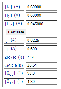
Let’s list the key configuration parameters:

• frequency=3.6MHz;
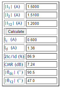
• drive voltages V1 and V2 are not perfectly balanced as detailed in the table below;
• other key parameters are listed in the table.

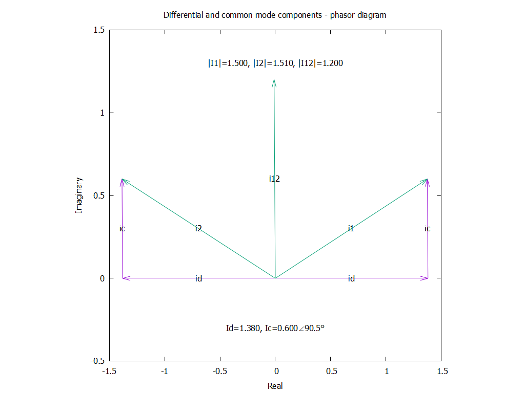
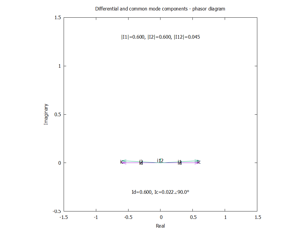
Above is a table showing for each configuration, the magnitude of the total common mode current |2Ic|, |2Ic| relative to the No balun baseline configuration, differential current |Id|, and |2Ic/Id| as a percentage.

Note that these currents are potentially standing waves, and they are measured at the antenna entrance panel, about 11 m of two wire feed line from the dipole feed point.

You might ask in respect of the total common mode current:

1. is the no balun result surprising?
2. is the current balun performance surprising?
3. is the voltage balun performance surprising?
4. does the measured CMRR of 29.2dB imply the reduction in common mode current due to the current balun of 24.3dB?
5. what does the measured CMRR infer?
6. can the CMRR be used in an NEC model of the system scenario?
7. can Zcm be used in an NEC model of the system scenario?

References

• Agilent. Feb 2009. Impedance Measurement 5989-9887EN.
• Agilent. Jul 2001. Advanced impedance measurement capability of the RF I-V method compared to the network analysis method 5988-0728EN.
• Anaren. May 2005. Measurement Techniques for Baluns.
• Skelton, R. Nov 2010. Measuring HF balun performance in QEX Nov 2010.

Dave Casler sets out in his Youtube video to answer why two wire transmission line has so little loss . With more than 10,000 views, 705 likes, it is popular, it must be correct… or is it?

He sets a bunch of limits to his analysis, excluding frequency and using lossless impedance transformation so that the system loss is entirely transmission line conductor loss.

He specified 300Ω characteristic impedance using 1.3mm copper and calculates the loop resistance, the only loss element he considers, to be 0.8Ω.

Above is Dave’s calculation. Using his figures, calculated \(Loss=\frac{P_{in}}{P_{out}}=\frac{100}{100-0.27}=1.0027\) or 0.012dB.

Above is my calculation of the DC resistance at 0.395Ω per side, so I quite agree with his 0.8Ω loop resistance… BUT it is the DC resistance, and the RF resistance will be significantly higher (skin effect and proximity effect).

Casler’s is a DC explanation.

Self taught mathematician Oliver Heaviside showed us how to calculate the loss in such a line.

Let’s calculate the loss for that scenario more correctly.

Above is the complete output from RF Two Wire Transmission Line Loss Calculator.

One of the results shows the values of distributed R, L, G and C per meter, and R is 0.486Ω/m or 14.81 for the 30.48m length, nearly 20 times Dave Casler’s 0.8Ω.

Unsurprisingly, the matched line loss is larger, calculated at 0.213dB, much higher than Dave Casler’s 0.12dB.

Now for a bunch of reasons, the scenario is unrealistic, but mainly:

• the conductor diameter is rather small, smaller than many 300Ω commercial lines and impractical for a DIY line; and
• two wire line is most commonly used with high standing wave ratio and the often ignored loss under the specific mismatch scenario is more relevant.

Conclusion

It is common that the loss in two wire line system underestimates the line loss under mismatch and impedance transformation that may be required as part of an antenna system.

Casler’s DC explanation appeals to lots of viewers, probably hams, and might indicate their competence in matters AC, much less RF.

… Read widely, question everything!

This article reports and analyses a user experiment measuring current in a problem antenna system two wire transmission line.

A common objective with two wire RF transmission lines is current balance, which means at any point along the transmission line, the current in one wire is exactly equal in magnitude and opposite in phase of that in the other wire.

Note that common mode current on feed lines is almost always a standing wave, and differential mode current on two wire feed lines is often a standing wave. Measurements at a single point might not give a complete picture, especially if taken near a minimum for either component.

MFJ-854

The correspondent had measured feed line currents using a MFJ-854.

Above is the MFJ-854. It is a calibrated clamp RF ammeter. The manual does not describe or even mention its application for measuring common mode current.

So, my correspondent had measured the current in each wire of a two wire transmission line, recording 1.50 and 1.51A. He formed the view that since the currents were almost equal, the line was well balanced.

I have not used one of these, I rely on my correspondents guided measurements. (I have used the instrument described at Measuring common mode current extensively.)

MFJ-835

This is the instrument that MFJ sell for showing transmission line balance. One often sees recommendations by owners on social media, it is quite popular.

If the needles cross within the vertical BalancedBarTM the balance is within 10%. If not, you know which line is unbalanced and by how much.

Note the quote uses current like it is a DC current, not an AC current with magnitude and phase.

So, in the scenario mentioned earlier, the needles would deflect to 50% and 50.3% on the 3A scale, the needles would cross right in the middle of the BalancedBarTM, excellent.

… or is it?

One more measurement with the MFJ-854

I asked the chap to not only measure the (magnitude) of the current in each wire, but to pinch the wires together and close the clamp around both and measure the current. The remeasured currents were of 1.50 and 1.51A in each of the two wires, the current in both wires bundled together was 1.2A.

What does this mean?

With a bit of high school maths using the Law of Cosines, we can resolve the three measured currents into common mode and differential mode components.

Above is the result, the current in each wire comprises a differential component of 1.38A and a common mode component of 0.6A. The common mode components in each wire are additive, so the total common mode current on the feed line is 1.2A.

Above is a phasor diagram of I1, I2 and I12, and the components Ic and Id.

Note in this diagram that whilst the magnitude of i1 and i2 are similar, they are not 180° out of phase and that gives rise to the relatively large sum I12 (the total common mode component of I1 and I2).

This is a severe imbalance, sufficient to indicate a significant problem and to prompt a physical and electrical check of the antenna and feed line conductors and insulators.

Repairs were made and the measured result was quite good.

Above are the measurements and calcs.

Above is the phasor diagram… a bit harder to read as there is very little common mode current.

By contrast with the previous case I1 and I2 are almost 180° out of phase and the sum of them, I12 has very small magnitude.

Conclusions

The MFJ-854 can be used effectively for measuring current balance.

Understanding the relative common mode and differential components hinted there was something very wrong in the antenna system.

Forget the MFJ-835 for proving balance. If the needles do not cross in the BalancedBarTM it indicates unbalanced amplitudes. If they do cross in the BalancedBarTM it indicates approximately balanced amplitude, but does not prove the phase relationship is approximately opposite and as shown in this example, is a quite erroneous result.