Jeff, K6JCA, kindly sent me a paper, (Dunsmore 1991) which gives design details for a variation of the common resistive Return Loss Bridge design.
This article expands on the discussion at Return Loss Bridge – some important details, exploring Dunsmore’s design.
Dunsmore’s design

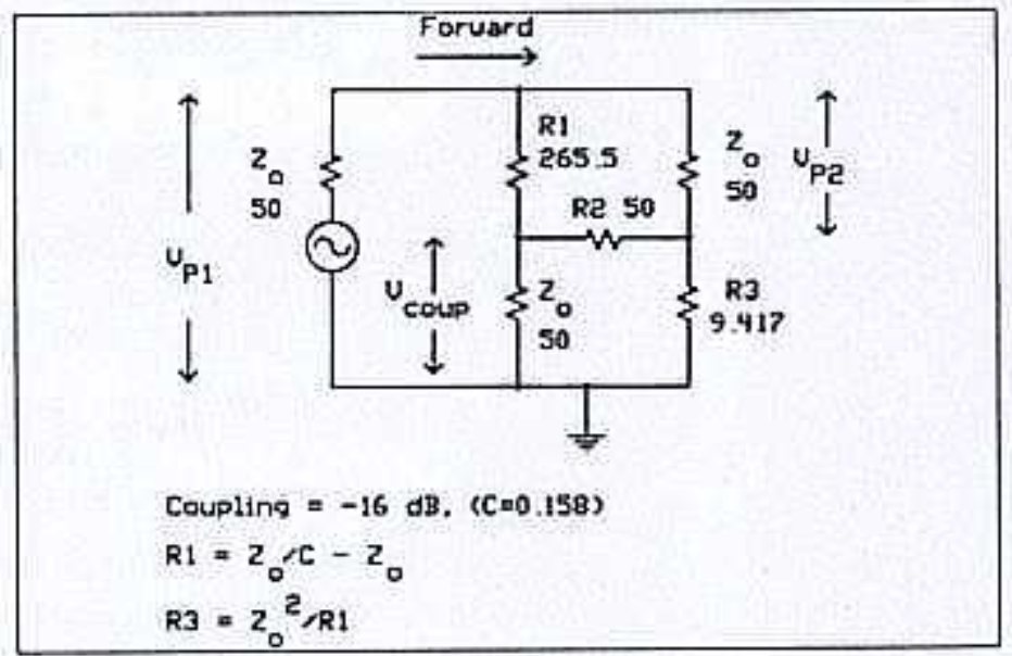
Above is Figure 3a from (Dunsmore 1991).
Exploration
The Dunsmore’s circuit has been rearranged to be similar to that used in my earlier articles.
Above is the rearranged schematic for discussion. It is similar to that used in the earlier article, but three components are renamed, R1, R2 and R3.
To analyse the circuit, we can use the mesh currents method. Mesh currents i1, i2 and i3 are annotated on the schematic.
The mesh equations are easy to write:
\(V_s=(zs+r1+r3) \cdot i1-r1 \cdot i2-r3 \cdot i3\\0=-r1 \cdot i1+(r1+r2+zd) \cdot i2-zd \cdot i3\\0=-r3 \cdot i1-zd \cdot i2+(r3+zd+zu) \cdot i3\\\)
This is a system of 3 linear simultaneous equations in three unknowns. In matrix notation:
\(\begin{vmatrix}i1\\i2\\i3 \end{vmatrix}=\begin{vmatrix}zs+r1+r3 & -r1 & -r3\\-r1 & r1+r2+zd & -zd\\-r3 & -zd & r3+zd+zu\end{vmatrix}^{-1} \times\begin{vmatrix}V_s\\0\\0\end{vmatrix}\\\)
Lets solve it in Python (since we are going to solve for some different input values) for Vs=1V.
First pass: zs, zref, zd are 50Ω, and zu is short circuit (1e-300 to avoid division by zero) for calibration and 25Ω for measurement. This example uses Dunmore’s 16dB coupling factor to derive the values for r1 and r3.
from scipy.optimize import minimize
import numpy as np
import cmath
import math

zs=50
zref=50
zd=50
c=0.5
c=10**(-16/20)
r3=zref/c-zref
r1=50
r2=zref**2/r3

print(c,r1,r2,r3)

#equations of mesh currents
#vs=(zs+r1+r3)⋅i1−r1⋅i2−r3⋅i3
#0=−r1⋅i1+(r1+r2+zd)⋅i2−zd⋅i3
#0=−r3⋅i1−zd⋅i2+(r3+zd+zu)⋅i3

#s/c cal
zu=1e-300
#solve mesh equations
A=[[zs+r1+r3,-r1,-r3],[-r1,r1+r2+zd,-zd],[-r3,-zd,r3+zd+zu]]
b=[1,0,0]
#print(A)
#print(b)
res=np.linalg.inv(A).dot(b)
#print(res)
vcal=(res[1]-res[2])*zd
#print(vcal)

#check oc
zu=1e300
#solve mesh equations
A=[[zs+r1+r3,-r1,-r3],[-r1,r1+r2+zd,-zd],[-r3,-zd,r3+zd+zu]]
b=[1,0,0]
#print(A)
#print(b)
res=np.linalg.inv(A).dot(b)
#print(res)
vm=(res[1]-res[2])*zd
#print(vm)
rl=-20*math.log10(abs(vm)/abs(vcal))
print('ReturnLoss (dB) {:0.2f}'.format(rl))

#check 25
zu=25
#solve mesh equations
A=[[zs+r1+r3,-r1,-r3],[-r1,r1+r2+zd,-zd],[-r3,-zd,r3+zd+zu]]
b=[1,0,0]
#print(A)
#print(b)
res=np.linalg.inv(A).dot(b)
print(res)
vm=(res[1]-res[2])*zd
#print(vm)
rl=-20*math.log10(abs(vm)/abs(vcal))
print('ReturnLoss (dB) {:0.2f}'.format(rl))
This gives calculated rl=9.54dB which is correct. Also ReturnLoss for OC reconciles with the SC calibration.
This result is sensitive to the value of Zs and Zd, changing them alters the result. It may be that there are other combinations of Zs, Zd, r1, r2, r3 that give correct results in all cases.
A common manifestation of design failure is that ReturnLoss of a short circuit termination will be significantly different to an open circuit termination, and the difference may be frequency dependent when combined with imperfections in the bridge.
Conclusions
Dunsmore gives an alternative design, though his formulas still depended on Zs=Zd=r1=Zref.
References
Dunsmore, J. Nov 1991. Simple SMT bridge circuit mimics ultra broadband coupler In RF Design, November 1991: 105-108.
Last update: 17th September, 2024, 7:08 PM