This article continues on from several articles that discussed the ARRL EFHW kit transformer, apparently made by hfkits.com, and the revised design at ARRL EFHW (hfkits.com) antenna kit transformer – revised design #1 – part 1.

This article presents a saturation calculation.

You will not often see saturation calcs (for reasons that will become apparent), though you will hear uninformed discussion promoting FUD (fear, uncertainty and doubt).

Lets assume that the core is capable of maximum continuous power dissipation of 10W (limited by factors like safe enclosure temperature, human safety, Curie point etc).

Now let’s estimate the magnetising current for 10W of core dissipation with 3t primary

Starting with the expected permeability above…

Gm is the magnetising conductance, the real part of Y above, 0.00231.

We can approximate the primary voltage for 10W core dissipation as \(V=(\frac{P}{G_m})^{0.5}=(\frac{10}{0.00231})^{0.5}=65.8V\) which implies 87W in a 50Ω load.

Magnetising current can be calculated at 10W core dissipation as \(I_m=\frac{V}{|Z|}=\frac{65.8}{222}=0.296A\)

In fact, under load, the net magnetising force may be just a little below 0.296A due to the effects of leakage inductance.

Let’s estimate saturation current for a 3t primary

Lets assume that under load, magnetising force due to current in the secondary offsets most of the magnetising force due to current in the primary and that the net magnetising force is due to magnetising current.

So, let’s solve.

Above is Fair-rite’s published data for their #43 mix (do not assume it applies to pretenders). Let’s take saturation flux density to be 1500 gauss, 0.15T.

Above is a calc of the saturation current for the 3t primary (peak), 4.01 Arms.

Conclusions

The saturation current is 14 times the magnetising current at 10W core dissipation, and is unlikely to be a significant limitation for low duty cycle modes.

This EFHW transformer is loss limited rather than saturation limited for most practical applications.

If you had in mind that this transformer was suited to peak power \(14^2 \cdot 87=17000 \text{ W}\) or more, then it may be driven into saturation.

Ian White gives the following diagram to explain what goes on at the coax to dipole junction.

He labels five currents in his explanation.

Let’s simplify that

Above is a diagram from Common mode current and coaxial feed lines showing the currents where a coax connects two two wires.

Lets morph that to the dipole feedpoint topology.

The whole thing is defined by just two currents, I1 and I2. The common mode current Ic=I1-I2. There is common mode current present in the short two wire connection to the dipole, and on the outer surface of the coaxial cable.

Note that I1, I2 and Ic are usually standing waves (ie they vary with location), and so these currents are defined here at the point where the conductors meet the end of the coax.

Are the currents measurable?

Using a clamp on RF current probe, the currents on the each of the two dipole conductors I1 and I2 is measurable, and so also the current on the outside surface of the coax shield Ic.

Remember also that these are sinusoidal AC currents, and I1, I2 and Ic refer to the magnitude of the currents.

The three currents can be resolved into the common mode and differential components, see Resolve measurement of I1, I2 and I12 into Ic and Id
(I12=Ic, the current measured with the probe around both two wire conductors or around the outside of the coax.

Can the currents be measured at an elevated dipole feed point?

Sure. I have done measurements of Ic over the length of coax by hoisting a current probe on a separate halyard to raise and lower it and reading it from the ground with a spotting scope.

Recall that Ic is usually a standing wave, and when you measure it at just one point, you don’t know much about it.

An example of the utter nonsense posted on social media.

My very first posting as a trainee was to Bringelly HF receiving station in 1970. It had Rhombic antennas every 30° of the compass, and a few other antennas, but the mainstay of operation was the set of Rhombics.

The nearby transmitting station at Doonside had a similar antenna arrangement of Rhombics fed with two or four wire open transmission lines to transmitters in a central building, for most operations, no coax involved between transmitters up to 30kW and antenna feed points.

Rhombics are an example of a non-resonant antenna, these were used for a large set of operating frequencies that were not harmonically related, were changed through the day with varying ionospheric conditions over the various circuits, within the broad frequency range of the Rhombics, and not restricted by a requirement for ‘resonant length’ of radiator conductors.

You do not have to look hard for other examples of non-resonant length radiators that have good radiation efficiency.

Yet hammy Sammy thinks that ‘resonance’, whatever it means, is a necessary condition for radiation efficiency.

In this case, the quote speaks to the credibility of the author.

Social media and errors

A further disadvantage of lots of social media platforms is the inability to edit mistakes. For example, one poster wrote in the same thread:

The qualitative conclusion here is that a “wild” impedance value of 890 – j418 which is far from resonance can and does yield an acceptable SWR.

My calc is that wrt 50Ω, that example has VSWR=21.7. We all make mistakes, but this appears locked in for perpetuity.

And of course it is unsociable to call out factual error on social media.

So what happened to Bringelly and Doonside?

Bringelly part of the new western Sydney airport and Doonside is a major road interchange (the Light Horse Interchange).

The NanoVNA can measure and display “phase”, is it useful for antenna optimisation?

Some authors pitch it as the magic metric, the thing they lacked with an ordinary SWR meter.

In a context where it seems most hams do not really have a sound understanding of complex numbers (and phase is one ‘dimension’ of a complex quantity like voltage, current, S parameters, impedance, admittance etc), lets look at it from the outside without getting into complex values (as much as possible).

The modern NanoVNA can display three phase quantities, only two are applicable to one port measurements as would commonly be done on an antenna system:

• s11 phase; and
• s11 Z phase.

Let’s look at a sweep of a real antenna system from the connector that would attach to the transmitter (this is the reference plane), plotting the two phase quantities s11 phase and s11 Z phase, and SWR (VSWR) and a Smith chart presentation of the s11 measurement.

Above is the measurement of the antenna system.

Like most simple antenna systems (this is a dipole, feedline, ATU), the most appropriate optimisation target is SWR, and minimum SWR well above 7.1MHz.

The SWR is 2.568 at the desired frequency, it is poor.

Do either or both of the phase plots give useful information on the problem, and leads to fix it?

s11 phase

s11 phase is -179.62° at the desired frequency (the marker).

Some authors insist optimal s11 phase is zero, some with a little more (and only a little more) knowledgeable insist it should be either 0° or 180°, take your pick. In fact the latter criteria essentially means the load impedance is purely resistive… but let’s deal with that under the more direct measurement s11 phase of Z.

Phase of -179.62° is approximately -180°=180°.

This metric is not very useful in this case.

s11 phase of Z

s11 phase of Z is -0.4°, approximately zero, which means the load impedance is almost purely resistive.

Of itself, s11 phase of Z does not identify the shortcoming.

So, what is the shortcoming?

If SWR is the optimisation target as proposed for this type of antenna, the SWR is poor, and the minimum is at a significantly higher frequency.

The SWR plot is revealing.

For more information, the value of Z is reported for the Smith chart marker as 19.47-j0.140Ω.

The reason that SWR is not 1.0 is that the feed point impedance is not exactly 50+j0Ω, and the main reason is that the real component is quite low at 19.47 and less importantly there is some very small reactance.

So, this provides information that to improve the match, the real component needs to increase significantly, and some minor trimming of the imaginary component.

Let’s make some matching adjustments

The sweep above is after some adjustment seeking to optimise the match.

Overall, the SWR plot shows that SWR is now fairly good at 7.1MHz, the Smith chart shows the marker just left of the prime centre so R is a little low and X is close to zero, the marker detail shows that Z is 45.57-j0.426Ω, so a little more information than the SWR curve, and with more resolution than reading the Smith chart graphically, R is a little low, X is close to zero. This is good information to guide the next matching steps if one wanted to refine the match.

The phase plots are of almost no value.

Conclusions

• Neither of the available s11 derived phase plots are of much use for this matching task.
• The SWR plot gives the best high level indication of the match.
• Knowledge of R and X components of Z can be helpful in understanding more detail of the match and guiding matching adjustments.
• This article has not explained the Smith chart in detail, it requires an understanding of complex quantities, so outside the scope and prerequisite knowledge set out for this article. In fact the Smith chart provides insight well beyond any and all of the other plots.

I see online discussion of specification bending radius for coax cables, and their application to ferrite cored common mode chokes.

A low Insertion VSWR high Zcm Guanella 1:1 balun for HF and follow on articles described a balun with focus on InsertionLoss.

Let’s remind ourselves of the internal layout of the uncompensated balun.

The coax is quality RG58A/U with solid polythene dielectric. The coax is wound with a bending radius of about 10mm, way less than Belden’s specified minimum bending radius of 50mm.

So, the question is does this cause significant centre conductor migration that will ruin the characteristic impedance:

• when it was first constructed; and
• through life.

Note the pigtails at each coax connector, they are a departure from Zo of the coax and the N type connectors. They can be seen as short sections of transmission line with Zo perhaps 200Ω or more. The effect of these is to transform impedance and so cause the input VSWR to depart from ideal.

When first constructed

Above is a chart from the original construction articles. InsertionVSWR @ 30MHz is about 1.15.

Note the pigtails at each coax connector, they are a departure from Zo of the coax and connectors. They can be seen as short sections of transmission line with Zo perhaps 200Ω or more. The effect of these is to transform impedance and so cause the input VSWR to depart from ideal.

After 5 years of service

This article presents measurement of the balun 5 years after it was made, 5 years in use, but not operated at temperatures above datasheet maximum.

As mentioned, the pigtails are the main contribution to InsertionVSWR. The balun was compensated using 10pF shunt capacitors at both coax connectors. (Possible compensation solutions were discussed at A low Insertion VSWR high Zcm Guanella 1:1 balun for HF – more detail #3).

Above is a NanoVNA screenshot of measurement of the compensated balun using the calibration LOAD, a couple of SMA(F)-N(M) adapters and a short SMA(M)-SMA(M) cable.

InsertionVSWR is highest at 1.01 @ 16MHz, at the limits of accuracy with this equipment. These 3kV 10pF ceramic capacitors have measured Q around 500 at 30MHz, expected loss is less than 200mW @ 1kW through.

The InsertionVSWR is not significantly affected by the quite small bending radius.

Voltage withstand

Does tight bending of this cable degrade voltage withstand of the balun?

Experience Hipot testing lots of baluns with this type of coax winding shows that the voltage withstand weakness is over the surface of the dielectric from braid to centre conductor, and pigtails of less than 15mm will flash over before internal flashover.

Alternative coax types

Coax with a solid PTFE dielectric is more suitable as the dielectric is harder and withstands higher temperatures before deformation.

Foamed dielectric cables are much more prone to migration of the centre conductor on tight bends, even at room temperature and are probably unsuitable for tight wraps.

Small diameter cables might seem the obvious answer, but they are higher in loss and will run at higher temperature.

Conclusions

Though the coax bend radius is substantially smaller than specification minimum bend radius:

• when first constructed, there was little evidence that the coax characteristic impedance was altered by the winding radius, and that the pigtails were the main contribution to InsertionVSWR; and
• after five years of service, the InsertionVSWR of the compensated balun is excellent, at the limits of accuracy of the test equipment and again, little evidence that the coax characteristic impedance was altered by the winding radius.

Solid dielectric coax may be quite satisfactory at static tight bend radius, subject to the temperature of operation and applied forces.

Jeff, K6JCA, kindly sent me a paper, (Dunsmore 1991) which gives design details for a variation of the common resistive Return Loss Bridge design.

This article expands on the discussion at Return Loss Bridge – some important details, exploring Dunsmore’s design.

Dunsmore’s design

Above is Figure 3a from (Dunsmore 1991).

Exploration

The Dunsmore’s circuit has been rearranged to be similar to that used in my earlier articles.

Above is the rearranged schematic for discussion. It is similar to that used in the earlier article, but three components are renamed, R1, R2 and R3.

To analyse the circuit, we can use the mesh currents method. Mesh currents i1, i2 and i3 are annotated on the schematic.

The mesh equations are easy to write:

This is a system of 3 linear simultaneous equations in three unknowns. In matrix notation:

Lets solve it in Python (since we are going to solve for some different input values) for Vs=1V.

First pass: zs, zref, zd are 50Ω, and zu is short circuit (1e-300 to avoid division by zero) for calibration and 25Ω for measurement. This example uses Dunmore’s 16dB coupling factor to derive the values for r1 and r3.

from scipy.optimize import minimize
import numpy as np
import cmath
import math

zs=50
zref=50
zd=50
c=0.5
c=10**(-16/20)
r3=zref/c-zref
r1=50
r2=zref**2/r3

print(c,r1,r2,r3)

#equations of mesh currents
#vs=(zs+r1+r3)⋅i1−r1⋅i2−r3⋅i3
#0=−r1⋅i1+(r1+r2+zd)⋅i2−zd⋅i3
#0=−r3⋅i1−zd⋅i2+(r3+zd+zu)⋅i3

#s/c cal
zu=1e-300
#solve mesh equations
A=[[zs+r1+r3,-r1,-r3],[-r1,r1+r2+zd,-zd],[-r3,-zd,r3+zd+zu]]
b=[1,0,0]
#print(A)
#print(b)
res=np.linalg.inv(A).dot(b)
#print(res)
vcal=(res[1]-res[2])*zd
#print(vcal)

#check oc
zu=1e300
#solve mesh equations
A=[[zs+r1+r3,-r1,-r3],[-r1,r1+r2+zd,-zd],[-r3,-zd,r3+zd+zu]]
b=[1,0,0]
#print(A)
#print(b)
res=np.linalg.inv(A).dot(b)
#print(res)
vm=(res[1]-res[2])*zd
#print(vm)
rl=-20*math.log10(abs(vm)/abs(vcal))
print('ReturnLoss (dB) {:0.2f}'.format(rl))

#check 25
zu=25
#solve mesh equations
A=[[zs+r1+r3,-r1,-r3],[-r1,r1+r2+zd,-zd],[-r3,-zd,r3+zd+zu]]
b=[1,0,0]
#print(A)
#print(b)
res=np.linalg.inv(A).dot(b)
print(res)
vm=(res[1]-res[2])*zd
#print(vm)
rl=-20*math.log10(abs(vm)/abs(vcal))
print('Zu: {:.2f}, ReturnLoss: (dB) {:.2f}'.format(zu,rl))

This gives calculated rl=9.54dB which is correct. Also ReturnLoss for OC reconciles with the SC calibration.

This result is sensitive to the value of Zs and Zd, changing them alters the result. It may be that there are other combinations of Zs, Zd, r1, r2, r3 that give correct results in all cases.

A common manifestation of design failure is that ReturnLoss of a short circuit termination will be significantly different to an open circuit termination, and the difference may be frequency dependent when combined with imperfections in the bridge.

RF Directional Bridge: Operation versus Source and Detector Impedances

Jeff, K6JCA, published a very interesting article RF Directional Bridge: Operation versus Source and Detector Impedances that is relevant to the wider understanding of Return Loss Bridges.

Conclusions

Dunsmore gives an alternative design, though his formulas still depended on Zs=Zd=r1=Zref.

References

Dunsmore, J. Nov 1991. Simple SMT bridge circuit mimics ultra broadband coupler In RF Design, November 1991: 105-108.

This article continues on from several articles that discussed the ARRL EFHW kit transformer, apparently made by hfkits.com.

This article presents a redesign of the transformer to address many of the issues that give rise to poor performance, and bench measurement of the prototype. Keep in mind that the end objective is an antenna SYSTEM and this is but a component of the system, a first step in understanding the system, particularly losses.

This is simply an experimental prototype, it is not presented as an optimal design, but rather an indication of what might be achieved if one approaches the problem with an open mind instead of simply copying a popular design.

• This prototype uses a Fair-rite 5943003801 core, equivalent in size to a FT240-43, it does not use NMG-H material (“Amidon 43”).
• A 3t primary is used, barely sufficient but a substantial improvement on the original 2t primary.
• The winding configuration is a primary of 3t and secondary of 21t, the secondary is close wound with 0.7mm ECW and the primary is wound using CAT5 cable wire wound over the middle of the secondary winding. This is done for two main reasons:
  • to permit some level of isolation of the ‘radiator’ and ‘counterpoise’ from the coax feed line with a view to reducing common mode current (most effective at the lower frequencies); and
  • to reduce leakage inductance with a view to improving broadband InsertionVSWR.

Leakage inductance

Leakage inductance is the enemy of broadband performance.

Total leakage inductance was assessed by measuring input impedance at 5MHz with the secondary shorted. Total leakage inductance is about 190nH (this slightly overestimates  leakage inductance due to resonance effects). This is two thirds that of the hfkits.com / ARRL original winding layout.

Through measurement with nominal load

The transformer is loaded with the nominal load comprising several 1% SMD resistors and VNA Port 2.

Above is a SimNEC design model, calibrated against measured input impedance with the nominal load.

Above is a pic of the measurement setup, a NanoVNA-H4 is to the right of the equipment shown. Note that the NanoVNA does not correct Port 2 mismatch error.

The transformers are described at Conversion of NOELEC style balun board to 1:1. The setup was SOLIT calibrated, the reference plane was the output side of the grey terminal blocks.

Above is a close up view of the prototype transformer with compensation capacitor. The loads are two 1% 2400Ω in parallel making 1200Ω, one in each secondary leg.

Measurement of the transformer was saved as a .s2p file.

Above is a SimNEC model importing the s2p file and adjusting for the voltage division of the 2400Ω and Port 2 impedance (assumed 50Ω, but uncorrected). The indicated Loss is just a little higher than predicted by the model, keep in mind that ferrites have quite wide tolerances.

Above is a plot of measured ReturnLoss and InsertionVSWR from the .s2p file.

Above is a plot of measured InsertionLoss from the .s2p file, and its components Loss and MismatchLoss. See Measurement of various loss quantities with a VNA for discussion of loss terms.

Common mode impedance

Mention was made that the common mode impedance may help to reduce common mode current at lower frequencies. Zcm will look like a small capacitance below 10MHz, of the order of 10pF for the layout shown. For that reason, I would not deploy an inductive common mode choke near to the transformer, put it at the other end of the feed line.

Conclusions

This is simply an experimental prototype, it is not presented as an optimal design, but rather an indication of what might be achieved if one approaches the problem with an open mind instead of simply copying a popular design.

The revised transformer has substantially better performance than the original: ARRL EFHW (hfkits.com) antenna kit transformer – measurement .

The modifications are mainly about:

• sufficient magnetising impedance; and
• reducing leakage inductance.

Loss remains a little higher than I would, an opportunity for the reader to find further improvement, a learning opportunity!

Jaycar’s LO1238 ferrite toroid is readily available in Australia at low cost and quite suits some HF RF projects.

The published data is near to useless, so a long time ago I measured some samples and created a table of complex permeability of the L15 material which I have used in many models over that time. It did concern me that measured µi was about 25% higher than spec, which is the limit of stated tolerance. Keep in mind that this is Chinese product with scant data published.

I have measured some samples purchased recently, and µi is closer to the specified 1000, so I intend using this new data in future projects.

Above is complex permeability calculated from s11 measurement of a single turn on the LO1238.

Downloads

L15.7z

Derivation of the expression for the unknown impedance in an s21 series through measurement arrives at the following expression:

\(Zu=(Zs+Zl)(\frac{1}{s_{21}}-1)\).

The diagram above is from (Agilent 2009) and illustrates the configuration of a series-through impedance measurement.

It is commonly assumed that Zs+Zl=100Ω, as is done in (Agilent 2001). That might be a reasonable assumption if the VNA correction scheme corrects source and load mismatch, but let’s consider the NanoVNA-H running NanoVNA-D v1.2.29 (Apr 2024) firmware (the current release).

It is good practice to validate a measurement system by measuring a known component. Let’s measure a 200Ω 1% resistor that measures 200.23Ω at DC (it is actually 2 x 0806 100Ω 1% resistors in series.

Above is the test setup, the SDR-kits test board fixture was SOLIT calibrated 1-31MHz using the parts shown at centre of the pic. The fixture is shown with a 200Ω 1% DUT that measures 200.23Ω at DC.

NanoVNA-H v3.3 with NanoVNA-D v1.2.29

Above is a screenshot from the NanoVNA-H measuring the SMD resistor that measures 200.23Ω at DC. The red and green traces use the internal feature to transform an S21 measurement into series thru impedance. The measured value of 204.9-j2.042Ω is significantly different to the expected 200.23Ω.

Above is a plot of calculated DUT assuming the Zs+Zl=100Ω (as does the screenshot above).  The measured values are significantly different to the expected 200.23Ω.

NanoVNA-D v1.2.29 does not correct source and load mismatch, and that is probably the main cause of the apparent error.

Lets turn the measurement around, if we measure some known impedance Zk, we can calculate Zs+Zl:

\(Zs+Zl=\frac{Zu}{(\frac{1}{s_{21}}-1)}\).

#import the network
nws21k=rf.Network(name+'-S21k.s2p')
zu=(50+50)*(1/nws21k.s[:,1,0]-1)
zk=200.23 #precision measurement of DUT resistor at DC
#calculate zs+zl using zu=(zs+zl)(1/s21-1) and zu=zk
zs_zl=zk/(1/nws21k.s[:,1,0]-1)

Above is a snippet of code in Jupyter to import the network and calculate the value of zs_zl (Zs+Zl) inferred by the s21 measurement of the DUT.

Above is a plotting of calculated zs_zl impedance components, real and imaginary, or R,X.

NanoVNA-H4 v4.3 with NanoVNA-D v1.2.40 using ERC

NanoVNA-D v1.2.40 (released 07/09/2024) includes optional Enhanced Response Correction which corrects source mismatch. The feature is turned on for these measurements.

The instrument was calibrated with a LOAD that measured 50.17Ω at DC, this was specified in the calibration.

The NanoVNA-H4 v4.3 has better Port 2 input impedance than the NanoVNA-H used in the previous tests.

All of these measures improve the accuracy of s21 series through measurement of Z.

Above is a screenshot from the NanoVNA-H4 measuring the SMD resistor that measures 200.23Ω at DC. The red and green traces use the internal feature to transform an S21 measurement into series thru impedance. The measured value of 199+j0.594Ω is different to the expected 200.23Ω, about 0.5%.

Above is a plot of calculated DUT assuming the Zs+Zl=100Ω (as does the screenshot above).  The measured values are significantly different to the expected 200.23Ω.

NanoVNA-D v1.2.40 does not correct load mismatch, and that is probably the main cause of the apparent error.

Lets turn the measurement around, if we measure some known impedance Zk, we can calculate Zs+Zl:

\(Zs+Zl=\frac{Zu}{(\frac{1}{s_{21}}-1)}\).

#import the network
nws21k=rf.Network(name+'-S21k.s2p')
zu=(50+50)*(1/nws21k.s[:,1,0]-1)
zk=200.23 #precision measurement of DUT resistor at DC
#calculate zs+zl using zu=(zs+zl)(1/s21-1) and zu=zk
zs_zl=zk/(1/nws21k.s[:,1,0]-1)

Above is a snippet of code in Jupyter to import the network and calculate the value of zs_zl (Zs+Zl) inferred by the s21 measurement of the DUT.

Above is a plotting of calculated zs_zl impedance components, real and imaginary, or R,X. Zs+Zl is considerably closer to ideal (100+j0Ω) than the previous case.

Conclusions

• The analysis here is specific to a NanoVNA-H v3.3 running NanoVNA-D v1.2.29 and NanoVNA-H4 v4.3 running NanoVNA-D v1.2.40 configured as described.
• The formula often given and implemented for transformation of a series through s21 measurement to impedance depends on an assumption that source and load ports have zero mismatch error (eg that any mismatch is corrected).
• NanoVNA-D v1.2.29 does not correct source and load mismatch, the results are mediocre.
• NanoVNA-D v1.2.40 combined with the improved NanoVNA-H4 v4.3 hardware does not correct load mismatch, but other improvements improve the accuracy.

References

• Agilent. Feb 2009. Impedance Measurement 5989-9887EN.
• Agilent. Jul 2001. Advanced impedance measurement capability of the RF I-V method compared to the network analysis method 5988-0728EN.

Fox Flasher MkII and several follow on articles described an animal deterrent based on a Chinese 8051 architecture microcontroller, the STC15F104E.

Fox flasher MkII update 7/2019 documented a rebuild of the enclosure etc.

This is an update after five more years operation outside.

Above is a pic of the device. The polycarbonate case has yellowed a little. Importantly the cheap PVA has not crazed, it is kept dry by the outer enclosure, and a hydrophobic vent helps keeps the interior dry.

The battery is a pouch LiPo single cell, it is in good condition. A previous trial with 18650 LiIon cells showed they were unsuitable for the environmentals.

Two previous articles were desk studies of the the ARRL EFHW kit transformer, apparently made by hfkits.com:

• Thoughts on the ARRL EFHW antenna kit transformer; and
• Thoughts on the ARRL EFHW antenna kit transformer – improvements?

This article documents a build and bench measurement of the component transformer’s performance, but keep in mind that the end objective is an antenna SYSTEM and this is but a component of the system, a first step in understanding the system, particularly losses.

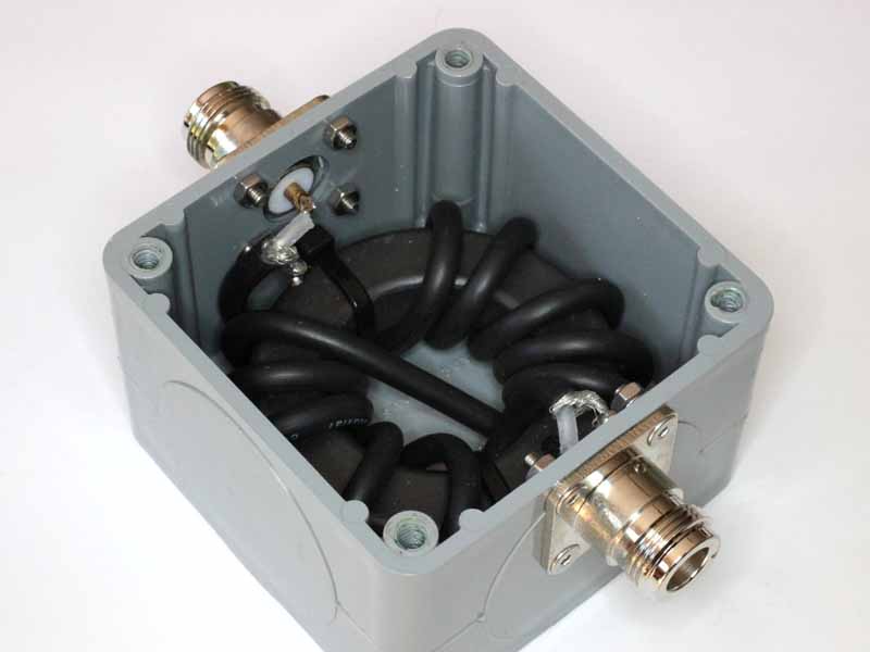
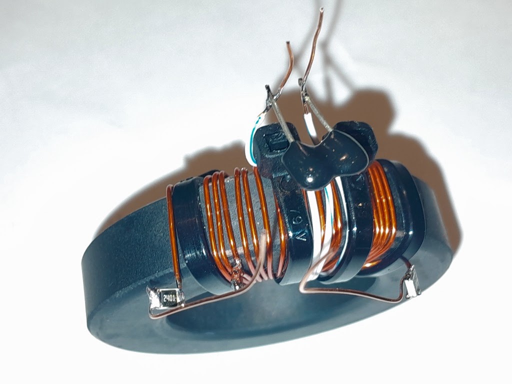
The prototype

Albert, KK7XO, purchased one of these kits from ARRL about 2021, and not satisfied with its performance, set about making some bench measurement of the transformer component.

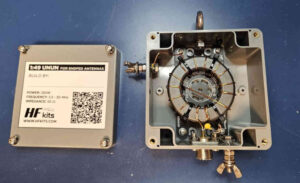
Above is Albert’s build of the transformer.

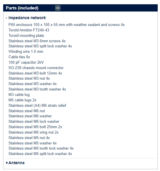
The kit parts list is as follows:

Magnetics

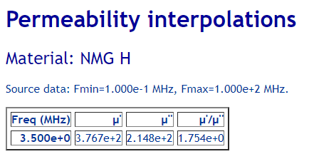
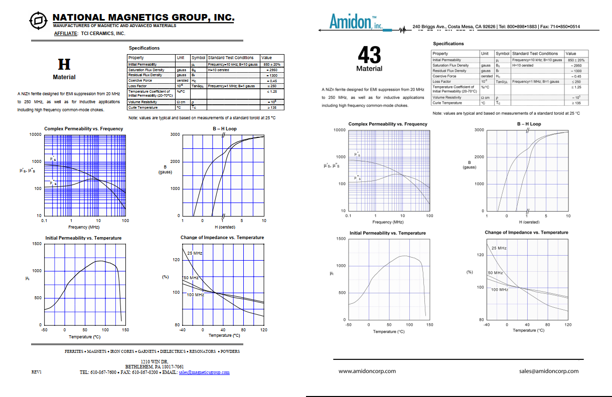
The first point to note is that Amidon’s 43 product of recent years has published characteristics that are a copy of National Magnetics Group H material (though they changed the letterhead).

Above is a side by side comparison of the NMG H material datasheet and Amidon 43, the Amidon appears to be a Photoshop treatment of the NMG.

Fair-rite have been a long term manufacturer of a material they designate 43 (which has changed over time), and it has been resold as such by many sellers. NMG H material is somewhat similar, but to imply it is equivalent to Fair-rite 43 might be a reach.

Overall design

I might note at the offset that the design is not original, there are countless articles on the net describing a 2:14 turn on a ‘FT240-43’ transformer for an EFHW using exactly the same winding layout.  As discussed in other articles on this site, 2t is insufficient for operation down to 3.5MHz using Fair-rite #43, even worse for the National Magnetics H material published as Amidon 43.

Measurement

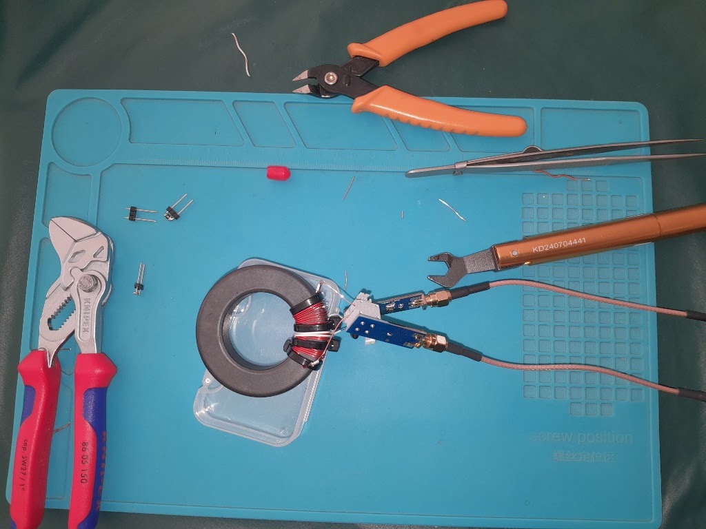
Measurements were made with a NanoVNA-H4. It is not a laboratory grade instrument, but well capable of qualifying this design and build.

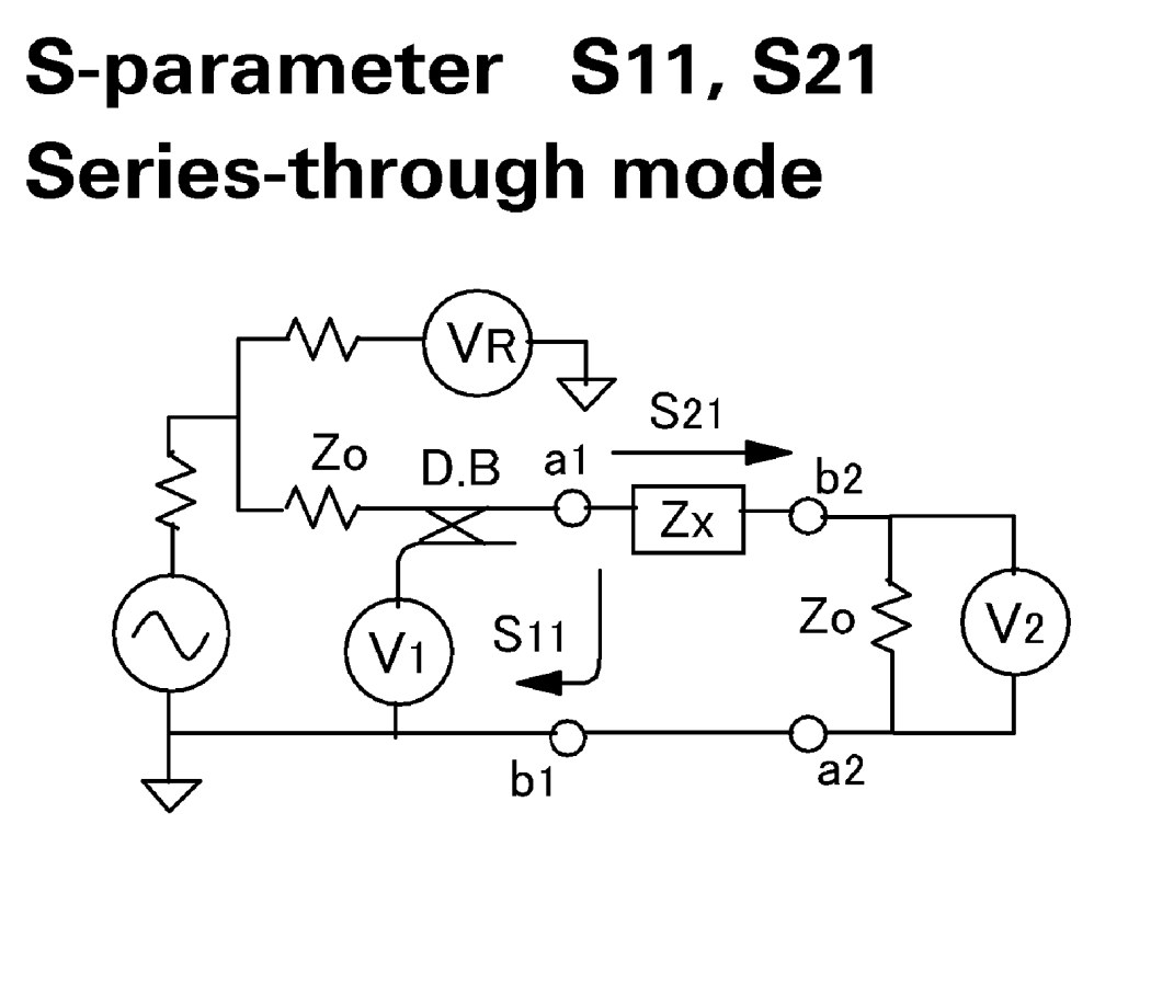
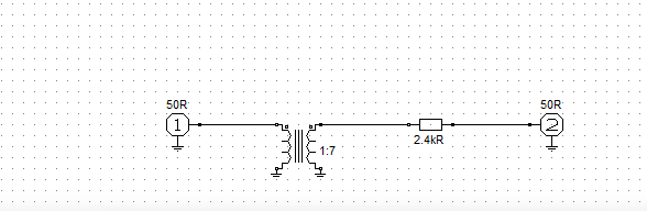
Albert performed a two port measurement using the setup above. This places a nominal load on the transformer, and the voltage division of the series resistor and Port 2 input impedance is used to correct the measured s21 figure.

So let’s take the measurements and calibrate a SimNEC model of the transformer.

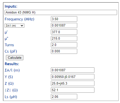
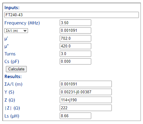
Above is the model using Fair-rite #43 material calibrated to measured leakage inductance and InsertionVSWR. The reconciliation of model (magenta) with measurement (green) is good. The equivalent Fair-rite part is 5943003801.

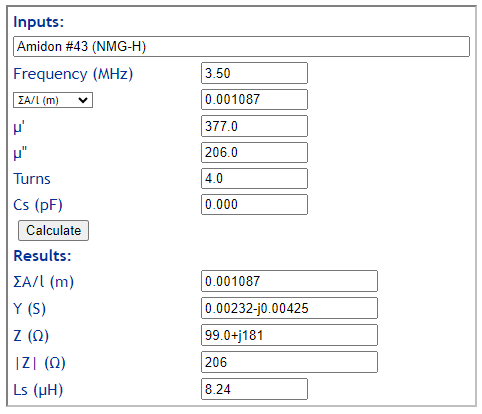
Let’s compare measurement to the same model but with Amidon 43 material (NMG-H):

Reconciliation is very poor at lower frequencies, the measured transformer appears to have significantly higher permeability.

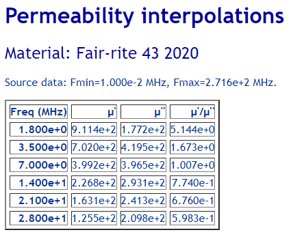
Measure core complex permeability

Let’s take a diversion for a moment and put this question to bed.

Above is complex permeability calculated from measurement of a 1t winding on the core used above compared with the Fair-rite #43 2020 published data. Keep in mind that tolerances on ferrite are relatively wide, these two reconcile very very well, there is no doubt in my mind that the material is Fair-rite #43. This questions the seller’s specified parts list.

A similar plot against NMG-H shows a stark difference.

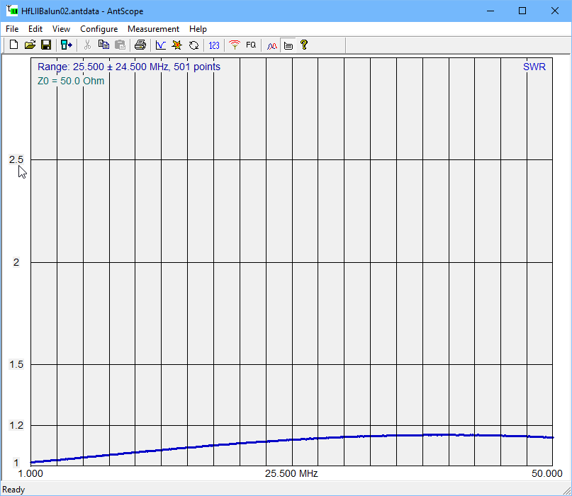
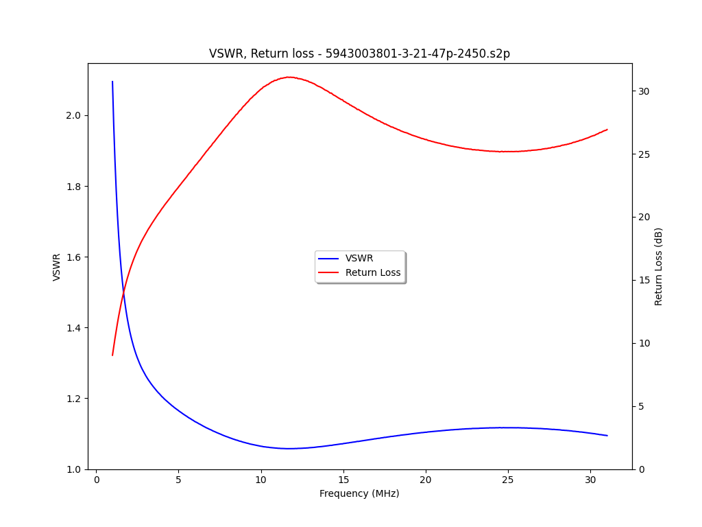
InsertionVSWR and ReturnLoss

So let’s return to the saved .s2p file from the two port measurement.

Above is a plot of bench measurement of ReturnLoss and (related) InsertionVSWR for the transformer with a nominal load.

The InsertionVSWR might look acceptable, but using InsertionVSWR as a single metric is a very limited view.

Above is a plot of InsertionLoss (-|s21|dB), and its components MismatchLoss and (Transmission) Loss. See Measurement of various loss quantities with a VNA for discussion of Loss terms.

Let’s dismiss performance below 7MHz, the plot shows it has insufficient turns.

Importantly, (Transmission) Loss is around 1dB at 7MHz, so 20% of the input power is converted to heat in the core and winding, mostly in the core. If you look back to the first SimNEC screenshot, the model predicts just under 1dB Loss, so measurement reconciles well with the prediction model.

Experience and measurement of Loss and thermographs informs that a transformer of this type in this type of enclosure is not capable of more than about 10W of continuous dissipation in typical deployments, less if it is in direct sun in a hot climate. That means the transformer is not likely to withstand more than about 50W average input power without damage or performance degradation.

Now that might be quite acceptable to some users, gauging by the number of web articles and Youtube videos recommending this, a lot of users apparently.

Credit

Credit to Albert for his interest in understanding these things, careful measurement of the prototype, and preparedness to dismantle the prototype for science.

Summary

So let’s end this article with the results of desk study and measurement:

• though the kit specifications state the core is Amidon #43, the sample kit is almost certain to contain a Fair-rite 43 core which is significantly different;
• two port measurement of the sample of one with nominal load showed around 1dB of Loss at 7MHz;
• MismatchLoss grows rapidly as frequency is reduced below 7MHz suggesting it has insufficient magnetising impedance, a result of insufficient turns;
• the winding configuration is not optimised for leakage inductance;
• popularity is not a good indicator of performance.

Where to from here?

These problems beg a redesign and measure of the transformer… more to follow.

It is often handy to have a reliable / known female UHF short and open circuit terminations when measuring using cables terminated in a UHF male connector.

This article describes a DIY solution.

Above is a diagram from Rosenberger showing the location of the ‘standard’ reference plane on UHF series connectors.

Above, the DIY short and open terminations. The short uses a M4x12 brass washer to short inner to outer at the connector body. This was measured using a VNA to have a one way propagation time of 50ps from the reference plane, and it is labelled for reference. The open termination simply has the pin cut off very close to the end of the dielectric, and again it measures 50ps.

These are not microwave standards, you are kidding yourself if you think you are making accurate measurements using UHF connectors above 100MHz, even less for demanding measurements.

You might wonder why you need an open termination. A UHF plug with a loose coupling sleeve and / or  exposed male pin is not a reliable open with known location.

An example application is measurement of the above transformer (though with nominal load of 2450Ω attached by very short wires) using a short cable from the VNA to the UHF(F) jack, If the cable + SC adapter described above is calibrated with an e-delay value that shows X=0 over a wide range of frequencies,  removing the short termination and connecting the cable to the transformer (with load) allows capture of the impedance as exists at the point that the (blue) compensation capacitor is attached, ie we want the reference plane to be the inboard end of the UHF connector. In this case, we ignore the 50ps offset.

One could take that s11 data and apply a small +ve or -ve capacitance in shunt to evaluate whether the optimal capacitor is larger or smaller and by how much.

Above is an example of measurement a correspondent’s build of a hfkits.com EFHW transformer (aka ARRL EFHW transformer) imported to the L element as a .s1p file with reference plane at the UHF connector, and Ccomp is an additional +/- adjustment dialled up and down to optimise the VSWR response. In this case an additional 20pF provided a small improvement to VSWR on the higher bands.

For this technique to be valid, it is essential that the reference plane be where the compensation capacitor will be applied.

You wanted a LOAD as well? See A check load for antenna analysers with UHF series socket. If you want a UHF(F) load, do the same thing but with a UHF(F)-SMA(F) adapter.

Derivation of the expression for the unknown impedance in an s21 series through measurement arrives at the following expression:

\(Zu=(Zs+Zl)(\frac{1}{s_{21}}-1)\).

The diagram above is from (Agilent 2009) and illustrates the configuration of a series-through impedance measurement.

It is commonly assumed that Zs+Zl=100Ω, as is done in (Agilent 2001). That might be a reasonable assumption if the VNA correction scheme corrects source and load mismatch, but let’s consider the NanoVNA-H running NanoVNA-D v1.2.29 (Apr 2024) firmware (the current release).

It is good practice to validate a measurement system by measuring a known component. Let’s measure a 200Ω 1% resistor that measures 200.23Ω at DC (it is actually 2 x 0806 100Ω 1% resistors in series.

Above is the test setup, the SDR-kits test board fixture was SOLIT calibrated 1-31MHz using the parts shown at centre of the pic. The fixture is shown with a 200Ω 1% DUT that measures 200.23Ω at DC.

Above is a screenshot from the NanoVNA-H measuring the SMD resistor that measures 200.23Ω at DC. The red and green traces use the internal feature to transform an S21 measurement into series thru impedance. The measured value of 204.9-j2.042Ω is significantly different to the expected 200.23Ω.

Above is a plot of calculated DUT assuming the Zs+Zl=100Ω (as does the screenshot above).  The measured values are significantly different to the expected 200.23Ω.

NanoVNA-D v1.2.29 does not correct source and load mismatch, and that is probably the main cause of the apparent error.

Lets turn the measurement around, if we measure some known impedance Zk, we can calculate Zs+Zl:

\(Zs+Zl=\frac{Zu}{(\frac{1}{s_{21}}-1)}\).

#import the network
nws21k=rf.Network(name+'-S21k.s2p')
zu=(50+50)*(1/nws21k.s[:,1,0]-1)
zk=200.23 #precision measurement of DUT resistor at DC
#calculate zs+zl using zu=(zs+zl)(1/s21-1) and zu=zk
zs_zl=zk/(1/nws21k.s[:,1,0]-1)

Above is a snippet of code in Jupyter to import the network and calculate the value of zs_zl (Zs+Zl) inferred by the s21 measurement of the DUT.

Above is a plotting of calculated zs_zl impedance components, real and imaginary, or R,X.

Conclusions

• The analysis here is specific to a NanoVNA-H v3.3 running NanoVNA-D v1.2.29.
• The formula often given and implemented for transformation of a series through s21 measurement to impedance depends on an assumption that source and load ports have zero mismatch error (eg that any mismatch is corrected).
• NanoVNA-D v1.2.29 does not correct source and load mismatch.

References

• Agilent. Feb 2009. Impedance Measurement 5989-9887EN.
• Agilent. Jul 2001. Advanced impedance measurement capability of the RF I-V method compared to the network analysis method 5988-0728EN.

This article is principally a short commendation for Jupyter or Interactive Python for ham radio related projects for the quantitative ham. Python is a cross platform programming language that has a very rich set of libraries to support scientific and engineering applications, and a good graph maker.

The exercise for this demonstration is to decompose three measurements of currents on a two wire transmission line at a point into the differential and common mode components at that point, and to plot a phasor diagram of a solution to the measurements. Remember that common mode current and differential current in an antenna system are usually standing waves.

Above is a diagram explaining the terms used, I1 and I2 are the magnitudes of currents in each conductor measured using a clamp on RF ammeter, and I12 is the magnitude of the current when both conductors are passed through the clamp on RF ammeter, i12 is the phasor sum of the underlying i1 and i2.

The solution to the problem lies in applying the Law of Cosines to find the angular relationship between the differential and common mode components, a high school trigonometry problem. In fact, we find the magnitude of the angle between ic and id.

Above is the solution, a phasor diagram taking id as the phase reference (ie 0°). Because we know only the magnitude of the angle between ic and id, there is a second possible solution as noted on the graphic.

Above is a screen capture of the Jupyter source cells and results.

When you look at the measurements that were taken, |i1| was within 2% of |i2| which many online experts would opine means there is nearly perfect balance. Measurement instruments based on simply comparing |i1| and |i2| indicating within the BalanceBar are deeply flawed… though very popular.

The decomposition shows that the magnitude of the differential current |id| is 25.7A and the magnitude of the total common mode current is 9.3A (4.65A per leg). It is not nearly balanced!

This demonstration uses high school mathematics applied to three measurements of current to drill down on the distribution of currents in a scenario that many would regard as balanced. Balanced means that the currents in each wire are equal but opposite in phase at any point along the line.

A quotation from Lord Kelvin:

When you can measure what you are speaking about, and express it in numbers, you know something about it. But when you cannot measure it, when you cannot express it in numbers, your knowledge is of a meagre and unsatisfactory kind. It may be the beginning of knowledge but you have scarcely in your thoughts advanced to the state of science.

The most common problem of broadband ferrite cored transformer designs for RF is insufficient turns which results in:

• low magnetising impedance Zmag causing:
• high InsertionLoss at lower frequencies;
• excessive core loss at low frequencies, and
• high InsertionVSWR at low frequencies.

This article give a simple test for a transformer that will have a nominally 50Ω input or output winding

Without going into a lot of magnetic and transformer theory, a through test using a VNA of the core and just one winding configured as a 1:1 (50Ω:50Ω) autotransformer is revealing. If that combination of turns, core, frequency is not adequate, it is very unlikely any transformer

Above is a schematic of the test configuration, the DUT is the central element, everything else is supplied by the VNA.

Above is an example mystery core with 3t for the 50Ω winding, connected in shunt with the through connection using a SDR-kits test board.

The test board and NanoVNA-H4 was SOLIT calibrated for the test, the the DUT inserted. For this core, the question is whether there are sufficient turns for 3.5MHz and up, we will test to 11MHz as this test will not reveal the high frequency limit, you need the other winding… which you can put on having established whether 3t is enough.

Above is the scan on the NanoVNA. Here we note that |s21| @ 3.5MHz is -0.528dB, this has potential. The network is symmetric, and so only a scan in one direction is needed.

Let’s import the .s2p file into SimNEC and do some calcs. (Where the .s2p file contains zeros for the s22 and s12 columns, SimNEC assumes a symmetric network and silently copies the values… which is ok as this network is symmetric.)

Above is the SimNEC model. The plots include calculated:

• InsertionLoss;
• Loss; and
• InsertionVSWR.

//Plots
dcl pfwd=S1.P/(1-(Gamma(S1.Z).M)^2);
LossdB=10*Log10(S1.P/L.P);
Plot(LossdB,"dB");
InsLossdB=10*Log10(pfwd/L.P);
Plot(InsLossdB,"dB");

Above is the code for these calculations. See Measurement of various loss quantities with a VNA for meanings of the terms. In this source case of UseZo(), pfwd=1, but it may not be for other source cases.

InsertionLoss @ 3.5MHz is 0.523dB, depending on the applications requirements, that might be acceptable, you probably would not want any worse.

Loss tells us about conversion of input RF power to heat, and it is relatively low at 0.083dB.

InsertionVSWR is moderately high at 1.9dB, again it depends on the application requirements.

Overall, this 1:1 (50Ω:50Ω) is likely to be marginal to unsuitable for most applications and would require at least 4t all else equal to perform reasonably well.

Now increasing the step up ratio typically degrades these parameters a little, so this test really identifies the minimum core / turns / frequency configuration that may result in an acceptable transformer with a higher step up ratio.

The discussion has inferred that the final transformer will be an auto transformer, but the analysis is useful for a conventional transformer using a medium to high µ core, just that a little more departure from the measured performance is likely with a high ratio conventional transformer.

So if such a test of the 50Ω winding and core has a bit of margin, wind the other winding and test the transformer.

7MHz and up

There are articles on this site that use this core (LO1238) with 3t 50Ω winding in 1:64 and 1:49 transformer configurations for an EFHW antenna system for 7MHz and up.

Whilst the combination doesn’t really make the grade at 3.5MHz, it does look better at 7MHz, see the chart above. Built, tested, measured transformers based on 3t winding worked well 7-30MHz (which suits lots of portable uses).

This is a follow up to Thoughts on the ARRL EFHW antenna kit transformer.

The first point to note is that Amidon’s 43 product of recent years is specified identically to National Magnetics Group H material. It is significantly different to Fair-rite’s 43 mix.

Though the parts list specifies an Amidon #43 core, I note that W1VT posted recently:

The ARRL kits don’t use Amidon parts as specified in the Parts List.

That was done as a “service” to those who wanted to know where to get parts for building their own without buying the kit.

The parts are sourced by a European company and shipped as kits to ARRL HQ, which acts as the distributor.

ARRLHQ publishes a Youtube video which shows a label by hfkits.com, and their website also lists Amidon FT240-43. hfkits.com may use a ‘genuine’ Amidon FT240-43 in their kits… this article applies to ‘modern’ Amidon FT240-43.

Trusting hfkits.com and ARRL, lets take the core as a ‘modern’ Amidon FT240-43 (equivalent to NMG-H).

Estimate the power dissipated in the core magnetised to 50V applied

Let’s make a first estimate of the power dissipated in the core with 50V impressed on the nominal 50Ω input winding alone (ie no secondary winding on the core), equivalent to 50W in 50Ω.

We  will calculate the magnetising admittance Gm+jBm, and the power dissipated is given by \(P=V^2G_m\).

Amidon 43 / National Magnetics H case

The first point to note is that Amidon’s 43 product of recent years is sourced from National Magnetics Group, and is their H material. It is not a good equivalent to Fair-rite’s 43 mix.

Let’s make a first estimate of core loss at 3.5MHz.

We can estimate the complex permeability which is needed for the next calculation.

The real part of Y is the magnetising conductance Gm (the inverse of the equivalent parallel resistance).

\(P_{core}=V^2G_m=50^2 \cdot 0.00950=23.8 \text{ W} \).

Amidon 43 / National Magnetics H case with 4t primary

Let’s recalculate with a 4t primary.

The real part of Y is the magnetising conductance Gm (the inverse of the equivalent parallel resistance).

\(P_{core}=V^2G_m=50^2 \cdot 0.00232=5.8 \text{ W} \).

To me, 5.8W core heating due to 50W RF input is a lot more acceptable that the 23.8W with a 2t primary. It is not stunning by an means but borderline acceptable. This configuration might stand 100W FT-8 without overheating (depending on the enclosure, environment etc).

So, can you use too many turns?

Yes, increasing the turns will increase leakage inductance which is a very important, if not most important, constraint on high end Insertion VSWR.

Try it and measure it.

Oh, but I only want to use 40m and up

You can follow the same process and estimate the minimum primary turns that suits your own acceptable core loss criteria.

One sees analyser sweeps of EFHW measurements posted online quite frequently, and a trend is that posters are quite pleased with the results.

Above is an example, a ‘user’s’ MyAntennas.com EFHW-4010 antenna with 23m of unspecified coax. Unfortunately it is a bit narrow, ordered up by an online expert.

The responses to the post were inevitably a focus on the location of the VSWR minima, and the value of VSWR at those locations.

But before focussing on the location of the resonances, I was taken with the rather compressed VSWR range. Let’s present that as ReturnLoss.

Above is ReturnLoss from the same .s1p file. For a shortish antenna, we might usually expect that the ReturnLoss minima will be quite a lot lower. Yes, these are out of band, but should not be dismissed as irrelevant.

Let’s look at an NEC model of a 21m long InvertedL EFHW.

Above is magnitude of Reflection Coefficient or ρ at the feedpoint (Zref=2450Ω) for a native EFHW as an Inverted L, ReturnLoss=-ρ (the chart is upside down compared to the previous one). Note that the ReturnLoss minima are up to about 1.2dB (recall that this model has no transformer loss, feed line loss, counterpoise on the ground loss).

The loss that results in high minimum ReturnLoss is likely to be a broaband loss, ie to affect in-band performance as well as between desired bands.

This begs the question, does the user’s antenna system contain some broadband loss mechanism that masks the natural impedance variation of the native EFHW?

If so, is there perhaps 2dB or more of broadband system loss that degrades RadiationEfficiency by as much as 40%.

Note also that there are fewer minima and maxima in the NEC model. The OP’s antenna with 5 distinct peaks shows signs of being electrically longer… the notion that the counterpoise is not part of the antenna length is wrong. So before focus on the location of ReturnLoss maximum (ie the ‘tuning’) there is an issue with the number of maxima and minima… this antenna is not working like a simple 40m EFHW on harmonics.

Background

From time to time, ham radio operators may question whether a section of installed and used coax is still good or significantly below spec and needs replacement.

A very common defect in coax installed outside is ingress of water. The earliest symptoms of water ingress are the result of corrosion of braid and possibly centre conductor, increasing conductor loss and therefore matched line loss (MLL). Any test for this must expose increased MLL to be effective.

Introduction

This article describes a simple but effective test of MLL for coax of known Z0 and length using a suitable one port antenna analyser (or VNA such as the NanoVNA), the nominal Z0 is sufficient to demonstrate cable is good.

The test involves measuring the resistance looking into a resonant length of coax with either an open circuit or short circuit termination.

The concept is to measure MLL and compare it to specification. Defects that increase MLL are not usually narrowband, but will be evidenced over a very wide range of frequencies so measurement at the exact operating frequency is not necessary.

Analyser requirements

Frequency

The analyser will need to cover a suitable frequency range for measurement. For cables for use on HF, I would advise measurement above 10MHz as actual Z0 is closer to nominal Z0. For higher frequencies, choose a range near to the operating frequency.

The analyser needs to be able to measure R and X reasonably accurately at a low impedance or high impedance resonance of the line section with either SC or OC termination.

Access

Access is needed to one end for the analyser, and at the other end for a SC or OC termination (the cable has to be disconnected from the antenna). It is not necessary to connect the ‘far end’ back to the analyser as you would for a two port transmission test.

Connectors

If you use connectors with a loose coupling sleeve (UHF, SMA etc), do not use a loose male connector as OC, connect it to a F-F adapter so nothing is loose.

To get accurate results, all connectors must be secure, clean and properly tightened.

Got all that under control? Let’s measure…

A practical example

The DUT is 10m of quite old budget RG58A/U fitted with crimp BNC connectors. A sample of this cable has previously been measured for braid coverage, it is just 78% so we might expect it to be a little poorer than Belden 8259.

Above, the top is a sample of the cable under test, and lower is Belden 8259. One can see the poorer braid coverage of the test cable… but does that alone condemn it?

The analyser is an AA-600 which uses an N(F) connector so a N(M)-BNC(F) adapter is used. The AA-600 uses a 16bit ADC, so it gives very good accuracy of extreme impedances (which is the case for this test).

Taking my own advice to measure above 10MHz, the third low impedance resonance of the cable section with OC termination is about 15MHz… let’s measure that.

Using the AA-600’s measure All facility and scrolling frequency up and down with the arrow keys until X passes through zero, we get the above measurements. I have taken a screen shot for the article, but no USB connection is needed for a practical measurement, just write down the frequency and R when X=0.

Now using Calculate transmission line Matched Line Loss from Rin of o/c or s/c resonant section we will calculate MLL (see Measuring matched line loss).

So, now we know the frequency of measurement and MLL, we need to find the specification MLL at that frequency using a GOOD line loss calculator.

Specification MLL is 0.06dB/m, we measured 0.07dB/m, it is a little higher than spec, probably a result of the budget construction, and no reason to condemn it, it is probably as good as the day it was made.

Can you use a NanoVNA?

Yes, you can any instrument that can measure R and X at resonance. I have demonstrated the technique using a noise bridge, an antenna impedance bridge (GR1606B), and a NanoVNA.

Conclusions

The technique and formulas used gives a practical simple but effective method of measuring matched line loss using a one port analyser (or any instrument that can measure R and X at resonance).

Several recent articles examined the use of s11 port extension or e-delay in some scenarios that might have surprised.

Recall that s11 port extension adjusts the measured phase of s11 based on the e-delay value converted to an equivalent phase at the measurement frequency.

It is:

1. an exact correction for any length of lossless line of Z0=50+j0Ω transmission line;
2. an approximate correction for a very low loss length of approximately 50Ω transmission line; and
3. an approximate correction for some specific scenarios such as those discussed at Some useful equivalences of very short very mismatched transmission lines – a practical demonstration.

Of course 1. does not exist in the real world, but 2. can give measurement results of acceptable accuracy if used within bounds. Both departures mentioned in 2. occur in the real world, non-zero loss and departure from Z0=50+j0Ω. Provided these departures are small, port extension may give acceptable results.

Let’s analyse some example measurements based on a 10m length of ordinary RG58A/U from 1-11MHz.

Above, measurement of the first series resonance with SC termination.

Note that the curve is a spiral inwards from the outer circle, the line is not lossless.

A requirement for e-delay to work well is that phase of s11 is proportional to frequency. This plot wraps, but apart from that, the plot looks approximately linear… however scale prevents detailed analysis.

Above, measurement of the first series resonance with OC termination.

Note that the curve is a spiral inwards from the outer circle, the line is not lossless.

Again the plot wraps, but apart from that, the plot looks approximately linear… however scale prevents detailed analysis.

Let’s find a value for e-delay at 1MHz and analyse the result.

Above is adjustment of e-delay to 115ns for approximately s11 phase 180° at 1MHz with SC termination.

The phase is correct at 1MHz, but at higher frequencies, it departs. So, the assumption that this TL has phase delay proportional to frequency is invalid. If you look closely, it is not a perfectly straight line, there is a small oscillation superimposed which is a sign of Z0 error. For these reasons, e-delay correction will have error.

Above is adjustment of e-delay to 100ns for approximately s11 phase 180° at 1MHz with OC termination.

The phase is correct at 1MHz, but at higher frequencies, it departs. So, the assumption that this TL has phase delay proportional to frequency is invalid. If you look closely, it is not a perfectly straight line, there is quite an oscillation superimposed which is a sign of Z0 error. For these reasons, e-delay correction will have error.

Let’s proceed anyway and look at the error. We will connect the 50+j0Ω termination load to the end of the cable and measure with each of the e-delays above.

Above is measurement of a 50+j0Ω termination with e-delay calibrated using 100ns e-delay (calibrated to OC termination). Note that the curve is a small circle, a sign of Z0 error and a hint that actual Z0 is about the centre of the circle plotted. Note though that Z0 is frequency dependent at these frequencies for this cable, so you can’t pin a pin on the chart and say this is Z0.

Above is measurement of a 50+j0Ω termination with e-delay calibrated using 115ns e-delay (calibrated to SC termination). Note that the curve is a small circle, a sign of Z0 error and a hint that actual Z0 is about the centre of the circle plotted. Note though that Z0 is frequency dependent at these frequencies for this cable, so you can’t pin a pin on the chart and say this is Z0.

At 5.75MHz and:

• e-delay from the SC calibration, Z=45.01+1.25Ω; whereas
• e-delay from the OC calibration, Z=45.01-1.26Ω.

For some purposes, that might be sufficient accuracy, for others it might be unacceptable:

• Z0 departure is more significant for lossier cables below about 10MHz; and
• in any event loss of tenths of a dB leads to measurable error.

Conclusions

Port extension or e-delay can provide a convenient means of shifting the reference plane given suitable test fixtures, but it is subject to significant error if the underlying assumption of lossless 50Ω line is breached.