Reading view

There are new articles available, click to refresh the page.

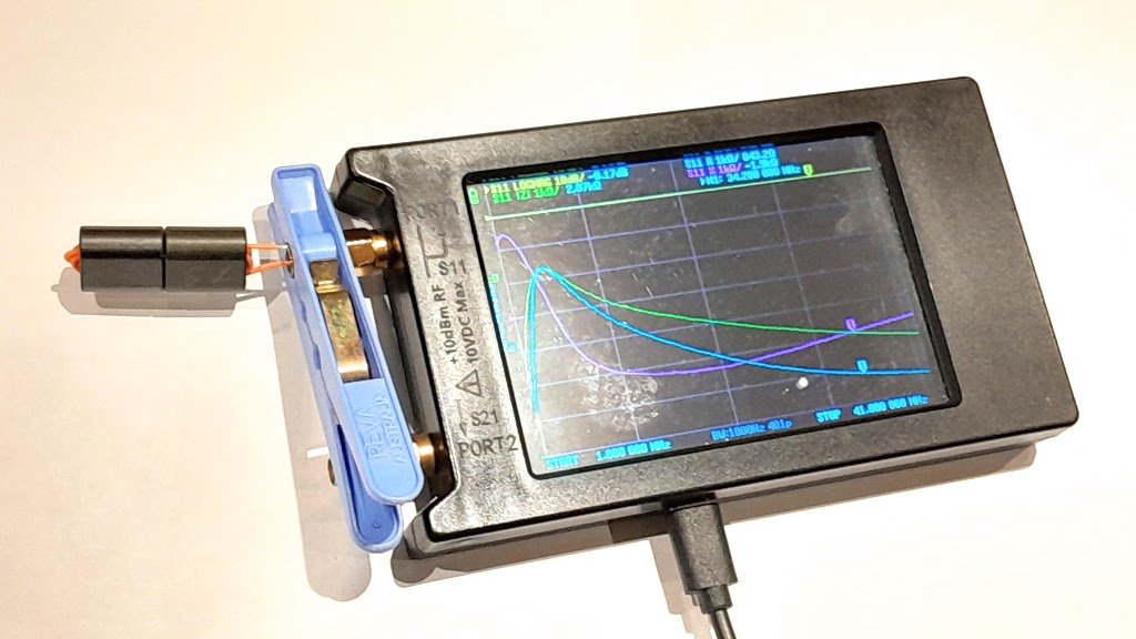
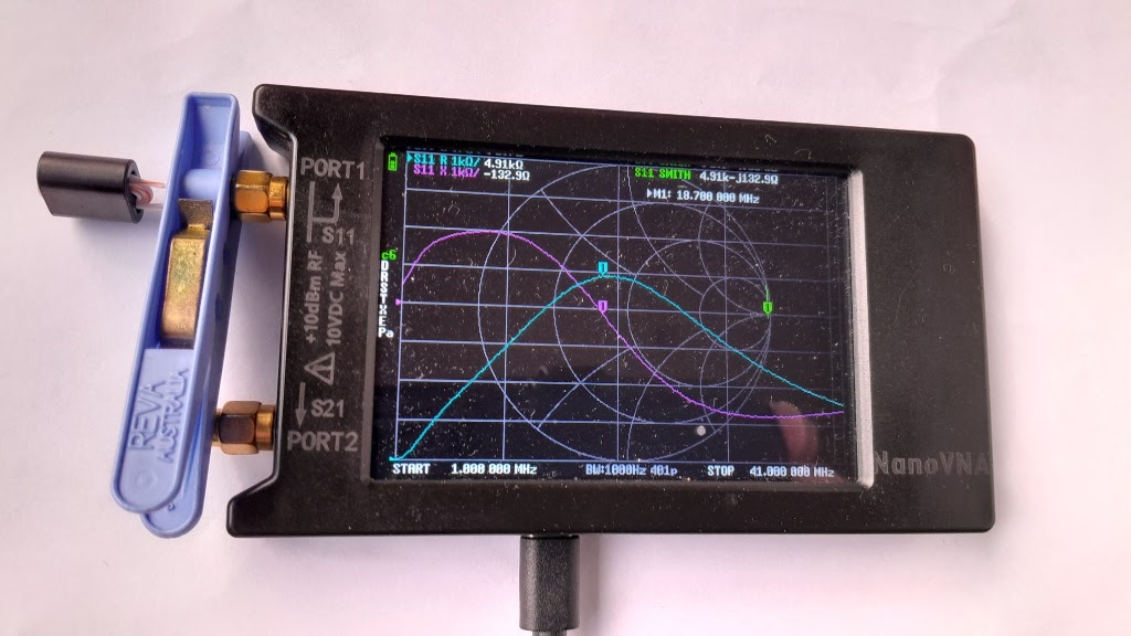
NanoVNA-H4 Bluetooth trial #1

This series of articles documents a trial of an Bluetooth link for remote operation of a NanoVNA-H4.

There are risks in fitting a radio transmitter in close proximity to RF measurement equipment. Those risks can be mitigated by just not doing it, but with care, it may be possible to achieve the utility of remote operation without degradation of the instrument.

The Bluetooth adapter is an external HC-05 adapter, <$5 on Aliexpress, configured for 38400bps.

The trial started with NanoVNA-D v1.2.35 firmware.

This should be straightforward as people claim to have this working.

Note than HC-05 modules are not all the same, and different performance may be obtained from different manufacturers products and different firmware versions. The one tested here was labelled hc01.com… but it is Chinese product and Chinese are copyists, it means little. Firmware reports version hc01.com v2.1.

AT+VERSION
+VERSION:hc01.comV2.1
OK

The module uses a CSR BC417 Bluetooth chip. The Windows end is unknown, but relatively new.

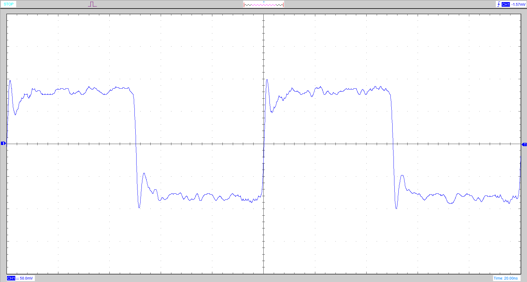
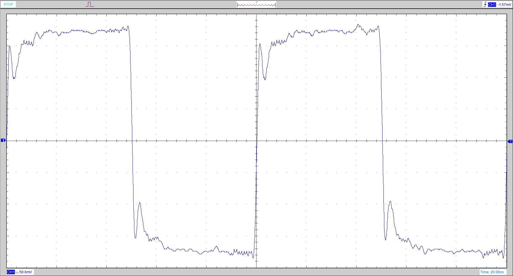
Some loopback throughput tests using Ezurio terminal

Above, results hint high protocol overhead.

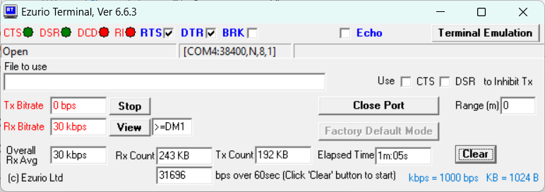
Above, close to ideal throughput for async encoding.

Problems encountered

System hangs sometimes

It sort of worked, but there was excessive delay in running a single scan from NanoVNA-App, though continuous scanning worked ok (after the same start up delay).

To help locate the problem:

  • a test was run of the UART connection to the VNA using a USB to serial adapter, so a wired connection; and
  • an extended bit error rate test was run on the Bluetooth link looped back at the HC-05.

Both comms links were reliable so the problem was the NanoVNA or NanoVNA-App.

Throughput at 38400 was 77%, quite close to the async encoding limit of 80%. Throughput at 230400 was 42%, not much better than half the async encoding limit of 80%.

A communications trace revealed that the NanoVNA appeared to hang on a pause command.

The issue was reported to Dislord, and the defect in NanoVNA-D v1.2.35 firmware fixed quite quickly (NanoVNA-D v1.2.37).

Downloading screenshots fails

I have a script set that are derived from a script published by Ho-Ro, and my script failed on the slow link.

That turned out to be a read timeout as the transfers are quite large, eg 307k which takes about 80s on an error free uncongested Bluetooth connection at 38400bps.

Higher speeds were tried, 115200bps failed, so I reverted to 38400bps which seems reliable.

In any event, the script needs facility to adjust timeout appropriately.

To do that, a baudrate parameter was added to the script, and it calculates a timeout equal to twice the time to transfer the calculated transfer size. If no baudrate is specified, it defaults to 1s timeout.

Here is the modified script.

#!/usr/bin/python
# SPDX-License-Identifier: GPL-3.0-or-later
'''
Command line tool to capture a screen shot from NanoVNA or tinySA
connect via USB serial, issue the command 'capture'
and fetch 320x240 or 480x320 rgb565 pixel.
These pixels are converted to rgb888 values
that are stored as an image (e.g. png)
'''

import argparse
from datetime import datetime
import serial
from serial.tools import list_ports
import struct
import sys
import numpy
from PIL import Image
import PIL.ImageOps
from pathlib import Path
import re

# ChibiOS/RT Virtual COM Port
VID = 0x0483 #1155
PID = 0x5740 #22336

app=Path(__file__).stem
print(f'{app}_v0.4')

# Get nanovna device automatically
def getdevice() -> str:
    device_list = list_ports.comports()
    for device in device_list:
        if device.vid == VID and device.pid == PID:
            return device
    raise OSError("device not found")

#extract default device name from script name
devicename=re.sub(r'capture_(.*)\.py',r'\1',(Path(__file__).name).lower())

# construct the argument parser and parse the arguments
ap = argparse.ArgumentParser()
ap.add_argument( '-b', '--baud', dest = 'baudrate',
    help = 'com port' )
ap.add_argument( '-c', '--com', dest = 'comport',
    help = 'com port' )
ap.add_argument( "-d", "--device",
    help="device type" )
ap.add_argument( "-o", "--out",
    help="write the data into file OUT" )
ap.add_argument( "-s", "--scale",
    help="scale image s*",default=2 )

options = ap.parse_args()
nanodevice = options.comport or getdevice()
if options.device!=None:
  devicename = options.device
outfile = options.out
sf=float(options.scale)

print(devicename)

if devicename == 'tinysa':
    width = 480
    height = 320
elif devicename == 'nanovnah':
    width = 320
    height = 240
elif devicename == 'tinysaultra': # 4" device
    width = 480
    height = 320
elif devicename == 'nanovnah4': # 4" device
    width = 480
    height = 320
elif devicename == 'tinypfa': # 4" device
    width = 480
    height = 320
else:
    sys.exit('Unknown device name.');

# NanoVNA sends captured image as 16 bit RGB565 pixel
size = width * height

crlf = b'\r\n'
prompt = b'ch> '

# do the communication
if(options.baudrate!=None):
  baudrate=int(options.baudrate)
  stimeout=int(size*2*2/baudrate*10)
else:
  baudrate=9600
  stimeout=1
print('Setting image donwload timeout to {0:d}s'.format(stimeout))
with serial.Serial( nanodevice, baudrate=baudrate, timeout=1 ) as nano_tiny: # open serial connection
    nano_tiny.write( b'pause\r' )  # stop screen update
    echo = nano_tiny.read_until( b'pause' + crlf + prompt ) # wait for completion
    #print( echo )
    nano_tiny.write( b'capture\r' )  # request screen capture
    echo = nano_tiny.read_until( b'capture' + crlf ) # wait for start of transfer
#    print( echo )
    nano_tiny.timeout=stimeout
    bytestream = nano_tiny.read( 2 * size )
#    print('bytestream ', len(bytestream))
    nano_tiny.timeout=1
    echo = nano_tiny.read_until( prompt ) # wait for cmd completion
#    print( echo )
    nano_tiny.write( b'resume\r' )  # resume the screen update
    echo = nano_tiny.read_until( b'resume' + crlf + prompt ) # wait for completion
    #print( echo )

if len( bytestream ) != 2 * size:
    print( 'capture error - wrong screen size?' )
    sys.exit()

# convert bytestream to 1D word array
rgb565 = struct.unpack( f'>{size}H', bytestream )

#create new image array
a=[0]*3
a=[a]*width
a=[a]*height
a=numpy.array(a, dtype=numpy.uint8)
for x in range (0,height):
  for y in range (0,width):
    index = y+width*x
    pixel = rgb565[index]
    a[x,y,0]=(pixel&0xf800)>>8
    a[x,y,1]=(pixel&0x07e0)>>3
    a[x,y,2]=(pixel&0x001f)<<3
image=Image.fromarray(a,"RGB")
#some transforms
image=image.resize((int(sf*width),int(sf*height)))
inverted_image=PIL.ImageOps.invert(image)
#save files
filename = options.out or datetime.now().strftime( f'{devicename}_%Y%m%d_%H%M%S' )
image.save(filename + '.png')
inverted_image.save(filename + 'i.png')

Note that the script picks up a default device name from the script name, so capture_nanovnah4.py defaults to nanovnah4 device type.
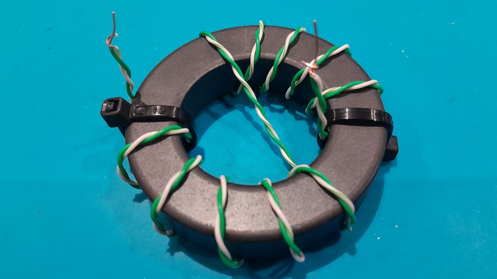
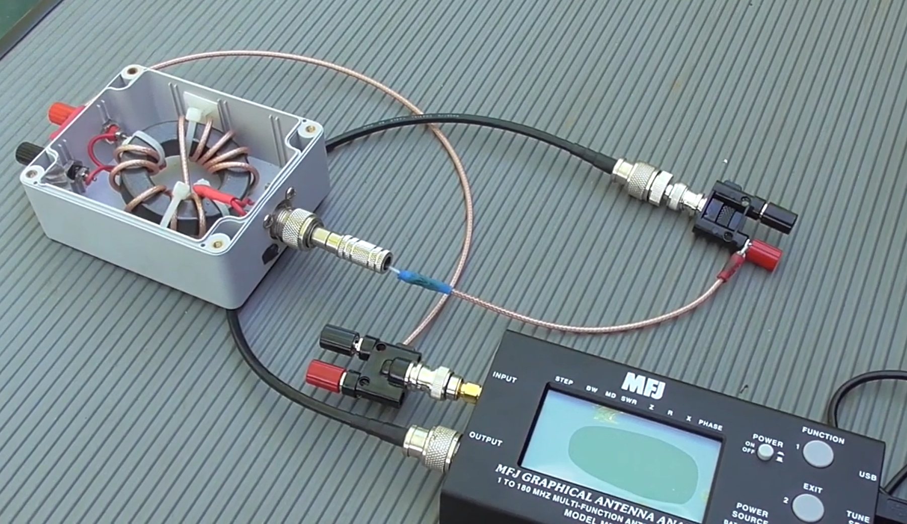
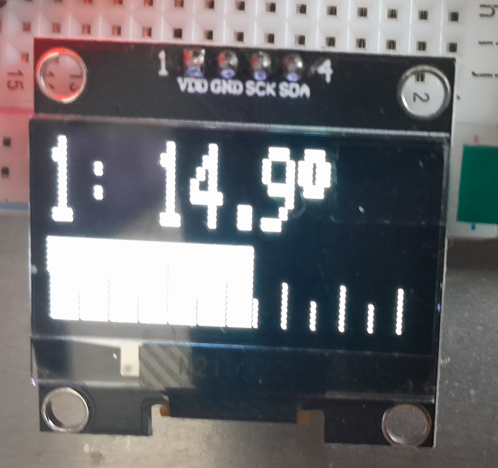
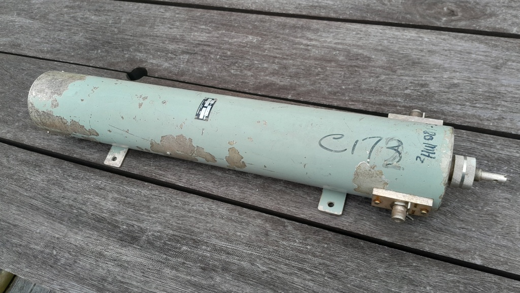
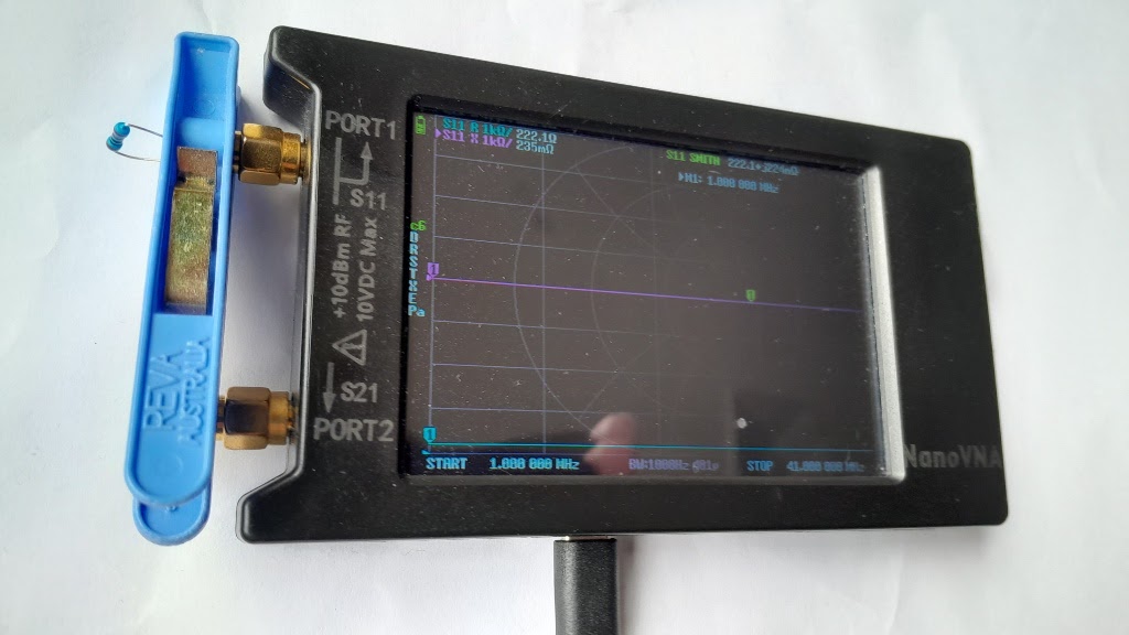
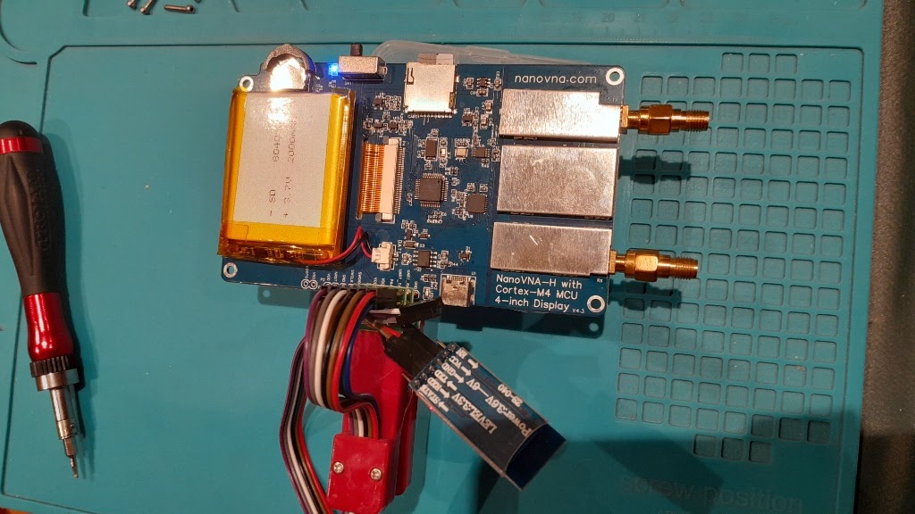
UART connector

For more convenient access to the UART pins, I installed a SIL 6w female header and cut a 3x18mm opening in the back for access.

Conclusions

This is not quite the no-brainer. The problems encountered were related to the specific firmware and my script (though Ho-Ro’s script may have the same issue). One is left wondering whether there were unresolved problems in some claimed implementations using this firmware.

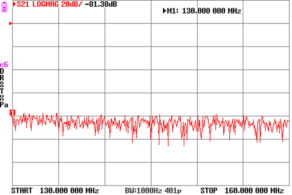
That said, the prototype appears to work ok. It now needs to be packaged and some tests made of EMC including noise floor degradation.

Last update: 14th July, 2024, 5:21 PM

Holzforma / Farmertec G395XP chainsaw – first impressions

I purchased a Holzforma G395XP chainsaw, it is a Chinese clone of the now discontinued Husqvarna 395XP It is a relatively old technology carburetted engine without stratified intake and without introducing electronic auto tune, a 30 year old design.

Some of the fasteners used to hold the top cowl down were noodled and would only work with a plain slotted screwdriver. They were replaced with hex button head screws.

In the light of experience with Holzforma / Farmertec G372XT chainsaw – early evaluation, a decision was made to preemptively vacuum and pressure test the G395XP saw.

It failed the vacuum test, not really badly, bad badly enough to warrant repair.

On removing the clutch etc to visibly examine the PTO side seal, the outer lip was not properly sitting on the shaft, the seal need to be driven in 1.0 to 1.5mm further. Given that the seals in the G372XT failed early due to one of both of low quality seal material and dry installation, the seal was removed and replaced. It was actually ok, not burnt, not worn, but had not properly engaged the shaft.

The flywheel was removed and the seal inspected, same problem but worse… the seal need to be driven about 2mm to properly engage the shaft. For the reasons given above, the seal was removed and a new one fitted.

A vacuum and pressure test was performed after 10min of operation with the new seals. There is a very slow leak of both vacuum and pressure, so slow as not to be concerning. It is substantially improved over the original hardly used crankshaft seals which were probably just not driven in sufficiently.

However, reassembling the muffler resulted in the M6 bolt thread stripping at just 6Nm (Husqvarna specified torque is 10-12Nm, hinting grade 8.8 fasteners), hinting low grade bolts on the Holzforma. A bad design where the expensive part (the bolt) fails  before the nut.

They were replaced with Husqvarna bolts, and new nuts.

Lessons learned

Some small problems, though the air leak (bad crankcase seal fitting) could quite quickly cause a hot seizure which would probably write the saw off.

I own two Holzforma saws, and both failed a crankcase vacuum test. I would probably not buy one again, but if I did, I would perform a crankcase vacuum and pressure test.

I would be reluctant to torque any fasteners to more than 50% of Husqvarna’s recommendation.

Evaluation post repairs

The saw starts easily, as easily as any big saw. After adjustment to service manual settings, idle is stable, WOT is stable. It is a heavy but powerful saw with it seems a moderately wide power band. Running on 50:1 Amsoil Sabre and Ethanol free ULP, it is fairly low smoke, not as clean as strato engines, but pretty good.

Last update: 12th July, 2024, 12:33 PM

Common mode choke measurement – length matters #2

Following on from Common mode choke measurement – length matters

Lots of people have reported experiments to show gross failure of s11 reflection measurement of high impedances such as those encountered measuring common mode chokes.

Above is a chart of a “10k resistor with leads” from (G4AKE 2020), the curve of interest is the s11 curve which he describes as unsuitable. He did not publish enough information to critique his measurement… so I will conduct a similar experiment.

My experiment

Above is a pic of my experimental setup. The resistor on Port 1 is a 10k 1% metal film resistor. The NanoVNA has been SOL calibrated at the Port 1 jack.

Above is a screenshot of the measurement. Quite similar result to that shown in (G4AKE 2020). (Note R, X, s11 phase at the marker.)

Note the s11 phase plot, we see the phase of s11 falling at a uniform rate from 1 to 101MHz.

What should we expect?

s11 for a 10k+j0 DUT should be 0.990050+j0 or 0.990050∠0.000° independent of frequency.

But we see this linearly decreasing phase. It is a big hint, transmission lines do this sort of thing.

So what if we attempt an approximate correction using e-delay.

e-delay of 54.5ps flattens the phase response, and the R and X values are closer to ideal, not perfect, but much closer than the uncompensated plot earlier.

A SimNEC simulation

Above is a SimNEC simulation of my experiment.

Conclusions

  • An experiment to duplicate G4AKE’s measurement achieves similar response.
  • Drilling down on the detail of the experiment response hints that the resistor pigtails contribute transmission line effect that are the main cause of the poor response.
  • An approximate compensation of the transmission line effects gives an impedance measurement that is much better than G4AKE’s recommended s21 series through measurement.
  • G4AKE condemns s11 impedance measurement as unsuitable, but there is good reason his fixture was the main reason for poor results… length matters.
  • Read widely, question everything.

References

Mar 2020. G4AKE. Measuring high and low impedance at RF.

Last update: 12th July, 2024, 7:57 AM

Common mode choke measurement – length matters

There must be thousands of Youtube videos of “how to measure a common mode choke” to give a picture of some sort of the test configuration… though most lack important detail… and detail IS important in this case. Likewise there are lots of web pages on the same subject, and some have pics of the test configuration, again mostly lacking important detail.

For the most part, these show test configurations or ‘fixtures’ that might be appropriate for audio frequencies, but are unsuitable at radio frequencies, even at HF.

Connecting wires at radio frequencies are rarely ideal, the introduce some impedance transformation that may or may not be significant to the measurement project at hand. Such connections can be thought of as transmission lines, often mismatched so they have standing waves (meaning the impedance of the load appears to vary along the line.

Let’s take the DUT in my recent article Baluns: you can learn by doing! as an example for discussion.

Let’s take the saved s1p file from a S11 reflection impedance measurement as the example.

Above is a plot of the common mode impedance of the choke, solid line is |Z|, dashed line is R, dotted line is X. This was measured with connecting wires <10mm, see the original article.

Now lets transform that to what we would see if just 100mm of 300Ω lossless line was used to connect the VNA to the balun.

The green curves are what would now be measured by the VNA. Observe the shift in the self resonant frequency (where X passes through zero), observe the shift in frequency of maximum |Z|, and the change in maximum |Z|.

These curves are like they were from different baluns.

Above is an example from a tutorial Youtube video by Fair-rite (a ferrite core manufacturer). Can you work out and draw a schematic of the test fixture? IIRC, the fixture itself was not calibrated, it cannot be because some of it is coax with the shield at one end disconnected.

A clear pic of the detail of all connections and how / where the fixture is calibrated is essential to interpreting any measurements.

A guide I often give people is this:

if you reduce the length of connections and measure a significant difference, then:

  • they were too long; and
  • they may still be too long.

Iterate until you cannot measure a significant difference.

Make some measurements with different fixture configurations, analyse the results and learn more about fixtures that you will glean from this or probably any written article or Youtube video.

If you believe s21 series through measurement technique or some other technique magically corrects poor fixtures, measure them and critically analyse the results… are they magic?

Read widely, question everything.

Last update: 11th July, 2024, 7:03 PM

Common mode choke measurement – estimating Cse

The article Baluns: you can learn by doing! presented measurements of a Guanella 1:1 Balun, a common mode choke.

Above is the prototype balun being a Fair-rite 5943003801 (FT240-43) wound with 11t of solid core twisted pair stripped from a CAT5 solid core LAN cable and wound in Reisert cross over style. Note that Amidon #43 (National Magnetics Groups H material) is significantly different to Fair-rite #43.

Above is a plot of the R and X components of Zcm taken from the .s1p file saved during measurement.

Note that it exhibits a self resonance at 13.5MHz. It is not simply an inductor, it is a resonator with an observed self resonant frequency (SRF) of 13.5MHz.

We can predict the impedance of the choke at low frequencies using the complex permeability, core parameters and turns, but as frequency approaches SRF some adjustment needs to be made to accommodate the self resonance. A simple adjustment is to shunt the simple inductor with some value of equivalent capacitance Cse that would cause the simple inductor to resonate at the observed SRF. This measure improves prediction of impedance up to SRF and a little higher depending on your accuracy requirement.

Above is a prediction based on µ, turns etc at the SRF. You will note that the calculated impedance is not consistent with resonance, but it can be used to calculate the Cse that would resonate it.

See also Ferrite permeability interpolations.

You could discover that Cse by inputting a value for Cse and iteratively increasing / decreasing it to find the value where the X part of Z passes through zero… but it is very tedious. You could use a hand calculator to find the value of C with B=0.0001116S.

Or you could use Solve Cse for self resonant inductor.

Above is calculation directly of Cse from calculated R, X at SRF and SRF. Note that you cannot measure R, X of the simple inductor as a practical inductor has the inseparable effects of self resonance, it comes as a bundle.

You could then return to the first calculator and enter the calculated value for Cse and so calculate the expected choke impedance etc.

Above, calculation of the choke using the calculated Cse. The calculated values to not reconcile exactly with measurement, measurement has errors, but worse, ferrites have quite wide tolerances.

Read widely, question everything.

Last update: 11th July, 2024, 2:33 PM

Dave Casler’s “why so little loss?”… a fact check!

Dave Casler sets out in his Youtube video to answer why two wire transmission line has so little loss . With more than 10,000 views, 705 likes, it is popular, it must be correct… or is it?

He sets a bunch of limits to his analysis, excluding frequency and using lossless impedance transformation so that the system loss is entirely transmission line conductor loss.

He specified 300Ω characteristic impedance using 1.3mm copper and calculates the loop resistance, the only loss element he considers, to be 0.8Ω.

Above is Dave’s calculation. Using his figures, calculated \(Loss=\frac{P_{in}}{P_{out}}=\frac{100}{100-0.27}=1.0027\) or 0.012dB.

Above is my calculation of the DC resistance at 0.395Ω per side, so I quite agree with his 0.8Ω loop resistance… BUT it is the DC resistance, and the RF resistance will be significantly higher (skin effect and proximity effect).

Casler’s is a DC explanation.

Self taught mathematician Oliver Heaviside showed us how to calculate the loss in such a line.

Let’s calculate the loss for that scenario more correctly.

Casler’s 1.3mm 300ohm two wire line

Parameters
Conductivity 5.800e+7 S/m
Rel permeability 1.000
Diameter 0.001300 m
Spacing 0.015000 m
Velocity factor 0.800
Loss tangent 0.000e+0
Frequency 14.000 MHz
Twist rate 0 t/m
Length 30.480 m
Zload 300.00+j0.00 Ω
Yload 0.003333+j0.000000 S
Results
Zo 301.80-j0.66 Ω
Velocity Factor 0.8000
Twist factor 1.0000
Rel permittivity 1.562
R, L, G, C 4.864062e-1, 1.261083e-6, 0.000000e+0, 1.384556e-11
Length 640.523 °, 11.179 ᶜ, 1.779231 λ, 30.480000 m, 1.271e+5 ps
Line Loss (matched) 0.213 dB
Line Loss 0.213 dB
Efficiency 95.21 %
Zin 3.031e+2-j1.940e+0 Ω
Yin 3.299e-3+j2.112e-5 S
VSWR(50)in, RL(50)in, MML(50)in 6.06, 2.892 dB 3.132 dB
Γ, ρ∠θ, RL, VSWR, MismatchLoss (source end) 2.183e-3-j2.105e-3, 0.003∠-43.9°, 50.364 dB, 1.01, 0.000 dB
Γ, ρ∠θ, RL, VSWR, MismatchLoss (load end) -2.990e-3+j1.096e-3, 0.003∠159.9°, 49.938 dB, 1.01, 0.000 dB
V2/V1 1.973e-1+j9.504e-1, 9.707e-1∠78.3°
I2/I1 2.055e-1+j9.590e-1, 9.808e-1∠77.9°
I2/V1 6.576e-4+j3.168e-3, 3.236e-3∠78.3°
V2/I1 6.164e+1+j2.877e+2, 2.942e+2∠77.9°
S11, S21 (50) 9.347e-1-j6.326e-2, 2.295e-2+j3.253e-1
Y11, Y21 8.345e-5+j6.986e-4, -1.011e-5-j3.385e-3
NEC NT NT t s t s 8.345e-5 6.986e-4 -1.011e-5 -3.385e-3 8.345e-5 6.986e-4 ‘ 30.480 m, 14.000 MHz
k1, k2 1.871e-6, 0.000e+0
C1, C2 5.916e-2, 0.000e+0
MHzft1, MHzft2 5.702e-2, 0.000e+0
MLL dB/m: cond, diel 0.006999, 0.000000
MLL dB/m @1MHz: cond, diel 0.001871, 0.000000
γ 8.058e-4+j3.676e-1


Above is the complete output from RF Two Wire Transmission Line Loss Calculator.

One of the results shows the values of distributed R, L, G and C per meter, and R is 0.486Ω/m or 14.81 for the 30.48m length, nearly 20 times Dave Casler’s 0.8Ω.

Unsurprisingly, the matched line loss is larger, calculated at 0.213dB, much higher than Dave Casler’s 0.12dB.

Now for a bunch of reasons, the scenario is unrealistic, but mainly:

  • the conductor diameter is rather small, smaller than many 300Ω commercial lines and impractical for a DIY line; and
  • two wire line is most commonly used with high standing wave ratio and the often ignored loss under the specific mismatch scenario is more relevant.

Conclusion

It is common that the loss in two wire line system underestimates the line loss under mismatch and impedance transformation that may be required as part of an antenna system.

Casler’s DC explanation appeals to lots of viewers, probably hams, and might indicate their competence in matters AC, much less RF.

… Read widely, question everything!


Last update: 9th July, 2024, 6:27 AM

Arduino thermometer using DS18B20 and OLED display

This article describes a Arduino based thermometer using a 1-wire DS18B20 digital temperature sensor using a SDD1306 or SH1106 OLED display.

The DS18B20 is a digital sensor, used for relative noise immunity, especially given the choice of an OLED display.

This is a basis for tinkering, for modification and a vehicle for learning.

Above is the sample display.

The code is written to support multiple sensors on the 1-wire bus, it cycles through each of the sensors displaying them for 1s each.

Parasitic power

The DS18B20 can be connected using a two wire connection and using “parasitic power”.

Above is a simple scheme for parasitic power which should work with one master and one sensor at the other end of the cable for tens of metres. For longer cables and multiple sensors, see (Maxim 2014).

Note that the Vdd pin is tied to ground.

1-Wire

Above is a capture of the DQ line for search and read of a single DS18B20.

Above is a zoomed in view of the 1-wire encoding format.

I2C display

The display uses I2C.

It takes just under 25ms to paint the display using the example code.

Source code

Here is source code that compiles in the Arduino IDE v2.3.2.

#define VERSION "0.02"
#include 
#define SCREEN_WIDTH 128 // OLED display width, in pixels
#define SCREEN_HEIGHT 32 // OLED display height, in pixels
#define TEMPMIN -20
#define BARGRAPH
#define PPD 2 //pixels per degree, must be +ve integer
#define TICKMIN 5
#define TICKMAJ 10
#define SSD1306_DISPLAY
//#define SH1106G_DISPLAY
#if defined(SSD1306_DISPLAY)
#define OLED_RESET    -1 // Reset pin # (or -1 if sharing Arduino reset pin)
#include 
Adafruit_SSD1306 display=Adafruit_SSD1306(SCREEN_WIDTH, SCREEN_HEIGHT, &Wire, OLED_RESET);
#endif
#if defined(SH1106G_DISPLAY)
#include 
#define WHITE SH110X_WHITE
#define BLACK SH110X_BLACK
Adafruit_SH1106G display=Adafruit_SH1106G(SCREEN_WIDTH,SCREEN_HEIGHT,&Wire);
#endif
#include 
DS18B20 ds(2);

#if defined(__AVR_ATmega328P__)
HardwareSerial &MySerial=Serial;
#endif

int i;
int barh=SCREEN_HEIGHT/2-2;
int basey=display.height()-1;
int tickh=barh/4;

void setup(){
  float adcref;
  long adcfs;

  #if defined(__AVR_ATmega328P__)
  analogReference(INTERNAL);
  adcref=1.10;
  adcfs=1024;
  #endif
  analogRead(A2); //Read ADC2
  delay (500); // Allow ADC to settle
  float vbat=analogRead(A2); //Read ADC again
  vbat=16*(vbat + 0.5)/(float)adcfs*adcref; //Calculate battery voltage scaled by 150k & 10k
  // Display startup screen
  MySerial.begin(9600);
  MySerial.println(F("Starting..."));
  #if defined(SSD1306_DISPLAY)
  display.begin(SSD1306_SWITCHCAPVCC, 0x3C);  //Initialize with the I2C address 0x3C.
  #endif
  #if defined(SH1106G_DISPLAY)
  display.begin(0x3C, true); // Address 0x3C default
  #endif
  display.setTextColor(WHITE);
  display.clearDisplay();
  display.setTextSize(1);
  display.setCursor(0, 0);
  display.print("DS18B20 thermometer");
  display.setCursor(0, 12);
  display.print("ardds18b20 ver: ");
  display.println(VERSION);
  display.print("vbat: ");
  display.println(vbat,1);
  display.display();
  delay(1000);
}

void loop(){
  int i,j;
  float temp;
  uint8_t id[8];
  char buf[27];

  j=1;
  while (ds.selectNext()){
    //for each sensor
    ds.getAddress(id);
    sprintf(buf," %02X:%02X:%02X:%02X:%02X:%02X:%02X:%02X ",id[0],id[1],id[2],id[3],id[4],id[5],id[6],id[7]);
    temp=(ds.getTempC());
    MySerial.print(j);
    MySerial.print(buf);
    MySerial.print(temp,2);
    MySerial.println(F(" °"));
    display.clearDisplay();
    display.setCursor (0,0);
    display.setTextSize(2);
    display.print(j);
    display.print(F(": "));
    display.print(temp,1);
    display.print((char)247);
    
    #if defined(BARGRAPH)
    int w=(temp-TEMPMIN)*PPD;
    //draw bar starting from left of screen:
    display.fillRect(0,display.height()-1-barh,w,barh,WHITE);
    display.fillRect(w+1,display.height()-barh-1,display.width()-w,barh,BLACK);
    //draw tick marks
    for(int i=0;i<SCREEN_WIDTH;i=i+PPD*TICKMIN) display.fillRect(i,basey-barh+3*tickh,1,barh-3*tickh,i>w?WHITE:BLACK);
    for(int i=0;i<SCREEN_WIDTH;i=i+PPD*TICKMAJ) display.fillRect(i,basey-barh+2*tickh,1,barh-2*tickh,i>w?WHITE:BLACK);
    if(TEMPMIN<0) display.fillRect((0-TEMPMIN)*PPD,basey-barh+tickh,1,barh-tickh,i>w?WHITE:BLACK);
    #endif

    display.display();
    j++;
    delay(1000);
    }
  delay(100);
  }

This code suits a 128*32 pixel display. Changes will be needed to optimise other display resolution.

Github repository

See https://github.com/owenduffy/ardds18b20 for code updates.

See https://github.com/owenduffy/tds18b20 for a platformio implementation.

References

Maxim. 2014. Guidelines for long 1-wire networks.

Last update: 7th July, 2024, 3:58 AM

NanoVNA examination of stacked ferrite cores of different mixes – more detail

NanoVNA examination of stacked ferrite cores of different mixes studied an example stacked core scenario, presenting measurements of a stack of BN43-202 and BN73-202, 5t wound through both.


The article stated:

They are somewhat similar (but only somewhat) to two series chokes with the same number of turns, so you might expect overlap of the responses.

Above is the measurement of the stacked configuration.

This article compares the stack with measurement of two series chokes of the same number of turns.

Above is the measurement of the series configuration.

They appear quite similar up to perhaps 5MHz or so, lets compare R, X on the same graph.

The magenta and cyan traces are R and X for the stacked configuration.

Below self resonance peaks, they are very similar which hints that the stacked cores are approximately the sum of responses of each of the cores at lowish frequencies, but as resonance comes into play, they differ.

It is clear that the stacked cores do not behave as equivalent chokes in parallel, that proposition is very wooly thinking.

This is measurement of a specific scenario, and the results cannot simply be extended to other scenarios. I have not (yet) been able to create a simple model of the stacked cores above self resonance, I would suggest that for reliability, any proposed configurations be measured. Whilst in this case, the series configuration appears to have a better impedance characteristic, that might not apply to other geometries and mixes.

Build, measure, learn.

Read widely, question everything.

Last update: 28th June, 2024, 8:48 AM

Effective measurement of common mode current on a two wire line – a user experience

This article reports and analyses a user experiment measuring current in a problem antenna system two wire transmission line.

A common objective with two wire RF transmission lines is current balance, which means at any point along the transmission line, the current in one wire is exactly equal in magnitude and opposite in phase of that in the other wire.

Note that common mode current on feed lines is almost always a standing wave, and differential mode current on two wire feed lines is often a standing wave. Measurements at a single point might not give a complete picture, especially if taken near a minimum for either component.

MFJ-854

The correspondent had measured feed line currents using a MFJ-854.

Above is the MFJ-854. It is a calibrated clamp RF ammeter. The manual does not describe or even mention its application for measuring common mode current.

So, my correspondent had measured the current in each wire of a two wire transmission line, recording 1.50 and 1.51A. He formed the view that since the currents were almost equal, the line was well balanced.

I have not used one of these, I rely on my correspondents guided measurements. (I have used the instrument described at Measuring common mode current extensively.)

MFJ-835

This is the instrument that MFJ sell for showing transmission line balance. One often sees recommendations by owners on social media, it is quite popular.


If the needles cross within the vertical BalancedBarTM the balance is within 10%. If not, you know which line is unbalanced and by how much.

Note the quote uses current like it is a DC current, not an AC current with magnitude and phase.

So, in the scenario mentioned earlier, the needles would deflect to 50% and 50.3% on the 3A scale, the needles would cross right in the middle of the BalancedBarTM, excellent.

… or is it?

One more measurement with the MFJ-854

I asked the chap to not only measure the (magnitude) of the current in each wire, but to pinch the wires together and close the clamp around both and measure the current. The remeasured currents were of 1.50 and 1.51A in each of the two wires, the current in both wires bundled together was 1.2A.

What does this mean?

With a bit of high school maths using the Law of Cosines, we can resolve the three measured currents into common mode and differential mode components.

Above is the result, the current in each wire comprises a differential component of 1.38A and a common mode component of 0.6A. The common mode components in each wire are additive, so the total common mode current on the feed line is 1.2A.

Above is a phasor diagram of I1, I2 and I12, and the components Ic and Id.

Note in this diagram that whilst the magnitude of i1 and i2 are similar, they are not 180° out of phase and that gives rise to the relatively large sum I12 (the total common mode component of I1 and I2).

This is a severe imbalance, sufficient to indicate a significant problem and to prompt a physical and electrical check of the antenna and feed line conductors and insulators.

Repairs were made and the measured result was quite good.

Above are the measurements and calcs.

Above is the phasor diagram… a bit harder to read as there is very little common mode current.

By contrast with the previous case I1 and I2 are almost 180° out of phase and the sum of them, I12 has very small magnitude.

Conclusions

The MFJ-854 can be used effectively for measuring current balance.

Understanding the relative common mode and differential components hinted there was something very wrong in the antenna system.

Forget the MFJ-835 for proving balance. If the needles do not cross in the BalancedBarTM it indicates unbalanced amplitudes. If they do cross in the BalancedBarTM it indicates approximately balanced amplitude, but does not prove the phase relationship is approximately opposite and as shown in this example, is a quite erroneous result.

Last update: 24th June, 2024, 9:00 AM

Dislord’s NanoVNA-D firmware v1.2.35 includes a facility to apply a correction based on the DC resistance of the LOAD

A recent series of articles discussed the question of how accurate does a calibration LOAD need to be.

Following on from that I requested a change to allow the actual resistance of LOAD to be used

These tests are not conducted in a temperature stable laboratory, so allow some latitude in results.

The NanoVNA-H running NanoVNA-D firmware v1.2.35 was SOL calibrated, but the calibration kit had a LOAD that measured 51.273Ω at DC using a high accuracy ohmmeter.

Above is an |s11| sweep after calibration. Measurement is limited by the instrument noise floor, about -80dB @ 1MHz. This says nothing about the load as it is based on a flawed calibration, but it shows us the noise floor. For reasonable accuracy, we might say here that we can measure |s11| down to about -70dB… subject to an accurate calibration LOAD.

Now that LOAD sets the instrument’s calibration reference impedance to 51.273Ω and if I was to measure a true 50Ω DUT, we would expect |s11|=-38dB.

I do not have a termination that is exactly 50Ω, so let’s measure another termination that measured 49.805 at DC using a high accuracy ohmmeter. We would expect the VNA based on the calibration above to show|s11|=-36.8dB.

Above is a screenshot of exactly that measurement, calibrated with 51.273Ω and measuring 49.805Ω, expect |s11|=-36.8dB and we get -36.6dB. That reconciles well.

Now lets specify the “Standard LOAD R”.

Above is a screenshot of the data entry.

Now with the correction applied, let’s measure the termination that measured 49.805 at DC using a high accuracy ohmmeter. We would expect the VNA to now show|s11|=-54.2dB.

Above is a screenshot of exactly that measurement, calibrated with 51.273Ω, “Standard LOAD R” correction applied for that value, and measuring 49.805Ω, expect |s11|=-54.2dB and we get -53.1dB. That reconciles well.

So what is the effective directivity with the “Standard LOAD R” correction?

If the measurement of the LOAD was without error, then the limit for low jitter measurement would be around 10dB above the noise floor measured earlier, so say |s11|=-70dB, which corresponds to ReturnLoss=70dB.

You could use that ReturnLoss as coupler Directivty in Calculate uncertainty of ReturnLoss and VSWR given coupler directivity to calculate uncertainty of a given measurement.

Above is a sample calculation.

But, measurement of LOAD has uncertainty.

Let’s say you measure LOAD with 1% uncertainty, and you measure 49.0Ω , but it could be as low as 48.5Ω (ie -1%), we can calculate the implied inherent ReturnLoss of the 48.5Ω using Calculate VSWR and Return Loss from Zload (or Yload or S11) and Zo) .

The LOAD could be specified as 48.5Ω with ReturnLoss=45dB.

So, entering “Standard LOAD R” is better than using the default 50Ω, but due to the uncertainty of measurement of that LOAD, the instrument Directivity is around 45dB. So, you can see that the accuracy of measurement of LOAD flows into the effective instrument Directivity which feeds calculation of s11 measurement uncertainty.

The instrument I used to measure the terminations has uncertainty of 0.035Ω on a 50Ω reading, which corresponds to a ReturnLoss of 69dB.

By contrast for example, a Fluke 106 has specified uncertainty of 1.1% at 50Ω which implies ReturnLoss 45dB… you are probably better just accepting 50Ω unless you know the LOAD is really bad.

SDR-kits sells relatively inexpensive calibration kits where they supply the measured DC resistance of LOAD.

Last update: 23rd June, 2024, 11:24 AM

NanoVNA examination of stacked ferrite cores of different mixes

A chap asked the assembled experts online:

Has anybody tried stacking say a type 43 on top of a 61 on top of a 31 for a wider bandwidth? Would the losses be any greater than using one toroid for each band?

There were some very firm assertions that this will not work well (without evidential support of course). Beware of firm assertions!

Quickly the case was compared to parallel chokes… and there is no parallel (pardon the pun), they are not the same.

They are somewhat similar (but only somewhat) to two series chokes with the same number of turns, so you might expect overlap of the responses. Two series chokes carry the same current and with the same number of turns apply the same magnetomotive force (mmf) to both magnetic cores.

But rather than hypothesise, even if from experience… lets measure.

Above is the DUT. It is a stack of BN43-202 and BN73-202, 5t wound through both. This is not two chokes in series, it is just like stacking a FT240-43 and FT240-73 in concept.

Above is the measured choke impedance from 1-41MHz.

It has an impedance profile that is the sum of the contribution of both cores, it is not a low impedance result. |Z|>2kΩ from 1-34MHz.

I will leave it to readers to measure 5t on each core type and compare them.

But fact does not often get in the way of energetic discussions on social media. Do we know what fact (or truth) is anymore?

I will do some thinking here…

One of the concerns was this will increase heat loss and reduce the power handling of the combination.

My analysis is that loss in ferrite is related to the flux, which is related to the current. Deployed in an antenna system, the combination has higher impedance which will often lead to lower current, reducing flux and heating.

I would argue that appropriate combinations of core mixes is capable of a broader band higher impedance profile, and improved power handling.

Build, measure, learn.

Read widely, question everything.

NanoVNA examination of stacked ferrite cores of different mixes – more detail


Last update: 28th June, 2024, 2:00 AM

NanoVNA measurement of a coaxial filter

This article discusses measurement of a coaxial filter. These are often referred to as “cavity filters”, but strictly speaking, a resonant cavity is different, these are a low loss transmission line section without input and output coupling.

The DUT is a single coaxial resonator configured as a band pass filter with adjustable separate coupling loops. The inside of this nearly quarter wave tube is a coaxial rod grounded at the right had end and almost reaching the left hand end with coupling loops attached to the coax connectors. The rod length is adjustable to tune it, everything is silver plated brass. The adjustable coupling loops allow some adjustment of bandwidth, but narrow bandwidth brings higher loss.

The filter is currently set for its tightest coupling, widest bandwidth, lowest loss.

It was last used for experiments to show that some ham grade receivers commonly used lack sufficient front end selectivity to deliver in the real world, the ‘shielded room’ performance stated in the specifications.

The instrument used here is a NanoVNA-H4 v4.3 and NanoVNA-D firmware NanoVNA.H4.v1.2.33.

It was SOLIT calibrated at the ends of 300mm RG400 patch leads on both ports. It was attached to the DUT with SMA(F)-N(M) adapters.

Let’s assess the NanoVNA s21 noise floor

Above is a plot of the noise in the s21 path, the noise floor is approximately -80dB, so measurements cannot be made with confidence down to about -70dB.

Whilst that noise floor probably permits measuring single stage rejection, especially with notches in duplexer filters, it is probably not sufficient to measure a cascade of two filter sections, much less three (which is a common configuration).

Now the measurement of s11 and s21

Above is a wide sweep from 130-160MHz (note the changed |s21| scale from the previous screenshot.

Above is a narrower sweep  over the ~3dB bandwidth. 3dB bandwidth is about 800kHz. ReturnLoss>20dB bandwidth (VSWR<1.2) is less than 100kHz (ReturnLoss=-|s11|.)

What if it had a notch filter as well?

We might expect that a notch would be 30dB to more than 50dB down. That is far enough above the |s21| noise floor to measure, but the notch of a cascade of filter sections will probably dip into the noise.

It might seem sufficient to measure the depth of notch in one stage of a filter, but thorough measurement requires assessment of the notch overall to demonstrate that they all line up on the correct frequency.

So, the often asked question…

Is this NanoVNA suitable for alignment and measuring performance of a typical repeater duplexer?

IMHO, no, it lacks sufficient dynamic range to measure the notch depths typically required.

Last update: 22nd June, 2024, 4:04 PM

Common mode choke measurement – for beginners

I have corresponded with many people trying to make valid measurements of a Guanella 1:1 balun, also known as a common mode choke.

In common mode, the device looks like a ferrite cored inductor. That might sound simple, but it is anything but, and it can be a challenge to measure.

There are lots of measures quoted, most of them IMHO are bogus or incomplete, usually specious… which accounts for their popularity.

This article focusses on making a valid measurement of the R and X components of the choke’s common mode impedance by the simplest means that is likely to give direct results.

Let’s start by proving the measurement instrument

I have taken an ordinary 1% metal film resistor and measured it with an accurate ohmmeter to be 221.4Ω. That is good, it reconciles with its markings. Now this is not a pure resistance at RF, it has some self inductance so we must expect to see that when measured with the VNA.

The wires are trimmed short. The bare end can be safely inserted into the centre pin of a SMA(F) jack.

One wire is poked into the Port 1 centre pin and the plastic clothes peg secures the other wire to the outside male threads of the SMA jack. Alternatively you could use a zip tie to secure the other wire to the outside male threads of the SMA jack.

Above, the test configuration.

Above, a screenshot. Focusing on the marker at 1MHz so that self inductance effects are small, we measure Z=222.1+j0.303. That reconciles well.

Now let’s move on to an unknown inductor

To simulate a small common mode choke, I have wound a Fair-rite 2843000202 (BN43-202) binocular core with 6t of single conductor stripped from an 4pr LAN cable. Note the specific core part, non-genuine parts may have different responses. The wires are trimmed short and 8mm of insulation stripped.

The bare end can be safely inserted into the centre pin of a SMA(F) jack.

Above is the test setup. One wire is poked into the Port 1 centre pin and the plastic clothes peg secures the other wire to the outside male threads of the SMA jack. Alternatively you could use a zip tie to secure the other wire to the outside male threads of the SMA jack.

The key thing is very short connections, they are less than 0.6° over the frequency range measured.

Here is a screenshot. The inductor is self resonant around 18.7MHz. The R and X curves are very similar to what you would get for a practical Guanella 1:1 balun though commonly the resonance would be somewhat lower, below 10MHz often. Narrower peaks will be observed with lower loss ferrite, eg #61 mix.

For the enquiring mind

If you have your own technique, fixture, test jig, cables etc try measuring a resistor like this and a choke like this (preferably exactly like this) by the method I have shown and your own technique and compare them.

Read widely, question everything.

Last update: 21st June, 2024, 8:53 AM

NanoVNA – how accurate does the LOAD need to be – part 3?

NanoVNA – how accurate does the LOAD need to be – part 2? answered the question in the context of an instrument that assumes the LOAD is exactly 50+j0Ω.

As mentioned in the article, there are more sophisticated models of the imperfection of nominal SHORT, OPEN and LOAD calibration parts (or ‘standards’), but the NanoVNA-H4 does not currently implement any of them.

A simple improvement is to accurately measure the DC resistance of the LOAD part, and use that resistance to calculate the expected LOAD response, and to use that in calculating the error terms that will be used in correction of raw measurements.

Precision Loads are expensive

LOADs with specified high ReturnLoss is an expensive option. Try to find a LOAD with ReturnLoss>40dB (VSWR<1.02)  for less than the price of the entire NanoVNA.

Roll your own

Another option is to buy some 0.1% 100Ω SMD resistors (50 for $7 on Aliexpress) and make a LOAD device that is suitable for calibration, but it is challenging to make such a lot that is good above say 100MHz.

Select for DC resistance

An option I have used is to buy a few inexpensive 6GHz Chinese terminations (~$6 ea) and measure their DC resistance, selecting the best as ‘good’ terminations. The best of a bunch of three I purchased had Rcd=49.085 which equates to RL50=54dB.

If the NanoVNA-H4 supported calibration based on DC resistance of the LOAD…

Some suppliers offer inexpensive calibration kits with measured DC resistance, eg SDR-KITS.

Some users may have a 4W ohmmeter that is capable of high accuracy measurement of loads, preferably to 0.1% uncertainty or better.

If the DC resistance was used during calibration / correction, then the instrument Directivity at frequencies below about 100MHz would be limited mainly by the instrument noise floor.

I have suggested such a facility to Dislord for NanoVNA-D so that its accuracy as a stand alone VNA can be improved.

See Dislord’s NanoVNA-D firmware v 1.2.35 includes a facility to apply a correction based on the DC resistance of the LOAD for implementation details.


Last update: 23rd June, 2024, 7:57 AM

NanoVNA – how accurate does the LOAD need to be – part 2?

This article continues on from NanoVNA – how accurate does the LOAD need to be – part 1?

Measures such as ReturnLoss, Gamma, s11, ro |s11|, VSWR are all wrt some reference impedance, often, but not necessarily 50+j0Ω.

The process of SOL calibration of a VNA, and its subsequent correction of DUT measurements, means that raw measurements are corrected with error terms that are derived from the calibration measurements and a set of responses expected of the calibration parts.

Those responses may be ideal responses; a simple short circuit (sc), a simple open circuit (oc) and an ideal load of some nominal value (say 50+j0Ω).

More sophisticated calibration may use a more accurate model for each of the SOL components, but NanoVNA uses simple ideal models for the SOL parts, including that L is 50+j0Ω.

So, if you use for example a 55Ω resistor for LOAD, then the correction factors are calculated to correct the raw measurement for a 55+j0Ω DUT to have \(s_{11}= \frac1{\infty}+\jmath 0\) (though noise will result is a lesser value, perhaps around 1e-40), and it its further computation assumes that s11 is wrt 50Ω, so it will render that DUT impedance as 50+j0Ω, ReturnLoss in dB as a very large number (perhaps 80dB).

If you did connect a DUT that was exactly 50+j0Ω, it will ‘correct’ the raw measurement to s11=-0.04762+j0, and it will render that DUT impedance as 45.45+j0Ω, ReturnLoss in dB as 26.4dB.

Saying it renders ReturnLoss as 26.4dB for an ideal 50+j0Ω DUT is equivalent to saying it has a Directivity (wrt 50Ω) of 26.4dB.

We can return to Calculate uncertainty of ReturnLoss and VSWR given coupler directivity and calculate the uncertainty of that system when it indicates for an unknown DUT, a ReturnLoss of say 21dB (equivalent to VSWR=1.2).

So for DUT with displayed ReturnLoss=21dB, actual ReturnLoss wrt 50Ω could be anywhere from 17.3dB to 27.7dB… quite a range!

So, to obtain a reasonably low uncertainty range, the Directivity of the instrument (the ReturnLoss of the LOAD calibration part) needs to be perhaps 10dB better than the DUT… use the calculator to try different instrument Directivity values and DUT measured ReturnLoss to find a combination with acceptable uncertainty.

So if you did want to measure ReturnLoss with uncertainty of less than 3dB, you might find the following works.

So, minimum coupler directivity is 32dB, you will need a LOAD calibration part that has ReturnLoss>32dB, equivalent to VSWR<1.05. That is a pretty practical component, and will not be outrageously expensive.

An exercise for the reader: what LOAD part ReturnLoss is needed to measure ReturnLoss of 30dB (VSWR=1.065) with less than 3dB uncertainty.

So, whilst you might see |s11| displays on your NanoVNA showing -30dB, they have very wide uncertainty unless the L calibration part is one of high accuracy.

Last update: 20th June, 2024, 9:21 AM

Verify coax cable performance with NanoVNA

This article walks through a simple verification of nominal 50Ω coax cable with connectors against manufacturer specifications using a NanoVNA.

The instrument used here is a NanoVNA-H4 v4.3 and NanoVNA-D firmware NanoVNA.H4.v1.2.33.

The DUT is a 10m length of budget RG58-A/U coax with crimped Kings BNC connectors, budget but reasonable quality. It was purchased around 1990 in the hey day of Thin Ethernet, and at a cost of around 10% of  Belden 8259, it was good value.

The notable thing is it has less braid coverage than 8259 which measures around 95%.

The cable has BNC(M) connectors, and BNC(F)-UHF(M) + UHF(F)-SMA(M) are used at both ends to simulate the impedance transformation typical of a cable with UHF(M) connectors.

Step 1: calibrate and verify the VNA

Note that |s11|<-40dB, or ReturnLoss>40dB. You really want at least 30dB ReturnLoss for this test to be as simple as described here.

The Smith chart plot of s11 is a very small spiral in the centre of the chart… approaching a dot.

Step 2: measure

The measurement fixture removed a ~150mm patch cable used during through calibration, so 750ps e-delay is configured on Port 2 to replace it. (one could just leave that cable in the test path and no e-delay compensation is needed).

Note that recent NanoVNA-D allows specification of e-delay separately for each port, don’t do as I have done if you use other firmware, leave the through calibration cable in place.

Above is a screenshot of the measurement from 1-31MHz.

Step 3: analysis

|s11|

Before rushing to the |s21| curve, let’s look at s11.

The Smith plot shows a small fuzzy spiral right in close to the chart centre, that is good.

The |s11| curve shows a periodic wave shape, lower than about -25dB. Recalling that ReturnLoss=‑|s11|, we can say ReturnLoss is greater than about 25dB. That is ok given the use of UHF connectors.

That wavy shape is mainly due to small reflections at the discontinuity due to the UHF connectors. They typically look like about 30mm of VF=0.67 transmission line of Zo=30Ω, so they create a small reflection. At some frequencies, the reflection from the far end discontinuity arrives in opposite phase with the near end reflection and they almost cancel, at other frequencies they almost fully reinforce, and in between they are well, in between… and you get the response shown in the screenshot. The longer the DUT, the closer the minima and maxima, and if the DUT is less than 180° electrical length, you will not see a fully developed pattern.

If you see a Smith chart spiral that is large and / or not centred on the chart centre, the cause could be that Zo of the DUT is not all that close to 50Ω, a low grade cable, possibly with migration of centre conductor or bunching of loose weave braid.

If your |s11| plot shows higher values, investigate them before considering the |s21| measurement. Check connectors are clean and properly mated / tightened.

|s21|

Now if that is all good, we can proceed to |s21|.

We can calculate InsertionLoss=‑|s21|, see Measurement of various loss quantities with a VNA.

It is interesting to decompose InsertionLoss into its components, because we may be more interested in the (Transmission) Loss component, the one responsible for conversion of RF energy to heat.

InsertionLoss for commercial coax cables is often specified as frequency dependent Matched Line Loss (MLL) or Attenuation (measured with a matched termination).

If InsertionLoss and MismatchLoss are expressed in dB, we can calculate \(Loss_{dB}=InsertionLoss_{dB}-MismatchLoss_{dB}\)

Above is a chart showing MismatchLoss vs ReturnLoss.  If ReturnLoss>20dB, MismatchLoss<0.05dB and can often be considered insignificant, ie ignored.

For example, the marker, ReturnLoss=26.05dB, so MismatchLoss is very small and can be ignored in this example and we can take that Loss≅InsertionLoss=‑|s21|.

We can calculate the MismatchLoss given |s11|:

As stated, at 0.011dB, it is much less than InsertionLoss so can be ignored.

So do we give this budget cable and connectors a pass?

At 15MHz, we can take MatchedLineLoss to be 6.8dB/100m which is a little higher than Belden 8259 datasheet’s 6.2dB/100m. That is not sufficient reason to FAIL the cable, we will give it a PASS.

Problem analysis

Let’s discuss a problem scenario to encourage some thinking.

Above is a through measurement after calibration.

What is wrong, shouldn’t |s11| be much smaller, shouldn’t the Smith chart plot be a dot in the centre?

Yes, they should.

If the calibration process was done completely and correctly, then this indicates that Zin of Port 2 is significantly different to the LOAD used for calibration. Note that they could BOTH be wrong. An approach to resolving this is to validate the LOAD, and when that is proven sufficiently accurate, remeasure Port 2 using a short through cable and check |s11|. If it is bad then perhaps a GOOD 10dB attenuator on Port 2 might improve things.

Now let’s ignore that problem and proceed to try the cable measurement (with that setup).

Above is a through measurement of an unknown 10m coax cable with 50Ω through connectors… no UHF connector issues here.

As before, look at |s11| first. The cyclic wavy nature hints that there is problem with one or more of LOAD, Port 2 Zin and DUT Zo. They should all be the same.

Note also the spiral Smith chart trace, if it is not centred on the centre of the chart, it hints that DUT Zo, LOAD and Port 2 Zin are significantly different.

So, to resolve this, one path is to validate the LOAD, and when that is proven sufficiently accurate, remeasure Port 2 using a short through cable and check |s11|. If it is bad then perhaps a GOOD 10dB attenuator on Port 2 might improve things. If these are both good, then the measurement suggests the DUT cable Zo is wrong.

The |s21| measurement is suspect until you resolve these issues.

Conclusions

Analysis of the |s11| measurement is important, good |s11| results are a prerequisite to analysing |s21|.

Comparison with manufacturers data gives a basis for PASS/FAIL.

Last update: 19th June, 2024, 3:08 PM

Toro ride-on mower fuel system blues

I have a Toro ride on mower (riding mower in North America) which I ran out of fuel when it was quite new (<1y) and having put 5l of fuel in the tank, it would not start after quite a bit of cranking.

In this instance, the battery failed. Prolonged cranking can buckle battery plates, or open intercell connecting links, and although this was prolonged cranking, it was not ridiculously long. Perhaps the battery was the real cause of the failure?

Nevertheless, I asked what I could do to prevent this recurring.

Well, with best intentions of never allowing the fuel to get low, it has run out of fuel a few times over 10y and has not restarted quickly, so was primed by injecting fuel into the carburettor hose.

Time for diagnostics

A note, the engine has been run on Ethanol free ULP, no Ethanol, ever.

Is the pump faulty?

This should not be the first question, but after market impulse fuel pumps are inexpensive and it is an easy test.

So, the pump was replaced and the old one dismantled and inspected. It was 2y old, and I was surprised that the valves were not as flexible as I expected… so maybe this is the problem.

Time showed the new pump was susceptible, time to do some logical analysis of the problem.

Is there an air leak that compromises pump performance when it is dry?

It is not easy to access the fuel tank end of the fuel hose, so as a shortcut, the hose was crimped off about 300mm from the fuel tank, the outlet hose removed from the fuel pump and a vacuum test conducted to check hoses, fuel filter, fuel pump.

That revealed a tendency for leaks at hose ends if the hose clamps were not applied over the barb or bulge in the nipple. Otherwise everything was good.

Note that air leaks are insidious, small air leaks may result in the engine running too lean at times, and that can cause expensive damage.

Perhaps that fixed the problem?

No.

A primer bulb

A primer bulb was inserted in the fuel line near to the tank. This allows for manually priming the carburettor after a fuel run-out… minimising long cranking and the risk of battery damage.

A 6mm primer bulb was purchased on Aliexpress for about $5.

Above, the primer was cut into the fuel line and the fuel line length adjusted so the primer bulb in suspended in air to avoid abrasion. The fuel line is zip tied to the wiring harness between filter and primer (not seen here due to the cross member).

The fuel line appears to be 6mm bore or perhaps 1/4″. 13.3mm (3/8 PEX) One-ear hose clamps were used to secure the hose.

The primer works fine, even with just a small amount of fuel in the tank, it takes quite a few squeezes to reach pressure.

One thing it will show is leaks upstream due to ineffective clamps… though note pressure tests the hose fitting in a more demanding way than the normal vacuum mode.

Last update: 19th June, 2024, 12:25 PM

NanoVNA-h4 v4.3 Port 1 waveform

This article documents the Port 1 waveform of my NanoVNA-h4 v4.3 which uses a MS5351M (Chinese competitor to the Si5351A) clock generator.

There are many variants of the NanoVNA ‘v1’, and most use a Si5351A or more recently a loose clone, and they will probably have similar output.

Above is the Port 1 waveform with 50+j0Ω load (power setting 0). By eye, it is about 3.3 divisions in the middle of each ‘pulse’. At 50mv/div, that is 165mVpp, 0.136W, -8.7dBm. The fundamental component (which is what is used for measurement below ~300MHz) is 3dB less, -11.7dBm.

Importantly, is is not a sine wave, it is a complex wave shape that is rich in harmonics. See square wave for more discussion.

Above is the Port 1 waveform with no load. By eye, it is about 6.6 divisions in the middle of each ‘pulse’. At 50mv/div, that is 330mVpp.

The voltage measurements are low precision, but suggest that if it behaves as a Thevenin source, since loaded voltage is half unloaded voltage, assuming that then Zsource=Zload=50+j0Ω.

How can you make good measurements with a square wave?

The instrument is mostly used to measure devices with frequency variable response, so how does that work (well)?

The NanoVNA-H is essentially a superheterodyne receiver that mixes the wave (send and received) with a local oscillator (LO) to obtain an intermediate frequency in the low kHz range, and digital filtering implements a bandpass response to reject the image response and reduce noise. So, whilst the transmitted wave is not a pure sine wave, indeed is rich in harmonics, the receiver is narrowband and selects the fundamental or harmonic of interest. The fundamental is used below about 300MHz, then the third harmonic is selected by the choice of the LO frequency above that, and still higher the fifth harmonic is selected.

Of course the power in the harmonics falls with increasing n which reduces the dynamic range of the instrument in harmonic modes. Though the NanoVNA adjusts power for the harmonic bands, one can observed a reduction in dynamic range.

How did you get those waveforms when it sweeps?

There is a stimulus mode labelled CW which causes output to be on a single frequency. In the sense that CW means continuous wave, and unmodulated sine wave, this is not CW but simply a single frequency approximately square wave. If you dial up 600MHz, the output is the fundamental 200MHz approximately square wave.

That is of little consequence if you use the NanoVNA’s receiver as a selective receiver, but if you use a broadband detector or power meter (which responds to the fundamental plus harmonic content), you may get quite misleading results.

The NanoVNA is not a good substitute for a traditional sweep generator that produced levelled sine waves of calibrated amplitude and had a source impedance close to 50+j0Ω

Last update: 18th June, 2024, 12:10 AM

Review of after market DeWalt compatible 18V 7Ah lithium-ion tool battery

I purchased on of these batteries on Big-W online for a mid-high price ($77), expensive enough compared to genuine to expect it would have near to rated capacity.

Above is a pic of the battery advertised. The delivered battery was labelled 7Ah.

They say a picture is worth a thousand words:

So, there it is, after three charge discharge cycles to develop full capacity, two measured discharge cycles. It measures <2Ah, <30% of rated capacity.

Full refund claimed, promptly processed by Big-W Online – return label within a few hours.

Last update: 17th June, 2024, 7:00 AM
❌