I wanted to have a fully open source solution to listen my radio(s) from my mobile phone and laptop over the web using a low cost Raspberry Pi as the rig control server. While there are many different remote station solutions out there I could not find one that would just work with a normal web browser (Chrome, Safari, etc) and without doing complicated network configurations exposing your internal WiFi network via a router. Also, I wanted to have the solution that is really easy to install to Raspberry Pi and update new versions as new features get added to the software.
I revisited the KX3 remote control project I did in Feb 2016 and started a new Cloudberry Live project. Cloudberry Live has several new improvements, such as no need to install Mumble client on your devices - you can just listen your radio(s) using a regular web browser. I did also upgrade my Amazon Alexa skill to leverage the ability to stream audio to Amazon Echo devices and control the frequency using voice commands.
Here is a short demo video how Cloudberry.live works:
Features
Listen your radio using web streaming from anywhere.
Web UI that works with mobile, tablet and laptop browsers (Chrome and Safari tested)
View top 10 DX cluster spots, switch the radio to the frequency with one click.
The software is currently at alpha stage - all the parts are working as shown in the demo above but need refactoring and general clean-up. The cloudberry.live proxy service is currently using a 3rd party open source proxy provider jprq. My plan is to host a reverse proxy myself in order to simplify the installation process.
The software is written using Python Flask framework and bash scripts. The deployment to Raspberry Pi is done using Ansible playbook that configures the environment correctly. I am using NGINX webserver to serve the web application.
The audio streaming portion is using HTTP Live Streaming (HLS) protocol and ffmpeg is used to stream audio from ALSA port and encode it using AAC format. There is a python http.server on port 8000 serving HLS traffic. I have tested Safari and Chrome browsers to be able to stream HLS audio. Chrome requires Play HLS M3u8 extension to be installed.
The home screen is shown below. This gives you the top 10 spots and a link to open audio streaming window. By clicking the frequency link on the freq column the server sends hamlib commands to the radio to set the frequency and mode. Only USB and LSB modes are supported in the current software version.
The Tune screen is shown below. This is still works-in-progress and needs some polishing. The Select Frequency allows to enter the frequency using numbers. The VFO range bar allows to change the radio frequency by dragging the green selection bar. The band selection buttons don't do anything at the moment.
The Configure Rig screen allows you to select your rig from the list of hamblib supported radios. I am using ICOM IC-7300 that is currently the default setting.
The Search button on the menu bar allows to check call sign from hamdb.org database. A pop-up window will show the station details:
Amazon Alexa Skill
I created a new Alexa Skill Cloudberry Live (not published yet) that uses the web API interface for selecting the frequency based on DX cluster spots and the HLS streaming to listen your radio. While the skill is currently using only my station, my goal would be to implement some sort of registration process so that Alexa users would have more choice to listen ham radio traffic from DX stations around the world using Cloudberry.live software.
This would give an opportunity also for people with disabilities to enjoy listening HF bands using voice controlled, low cost ($20 - $35) smart speakers. By keeping your radio (Raspberry Pi server) online you could help to grow the ham community.
Installation
I have posted the software to Github in a private repo. The software will have the following key features
One step software installation to Raspberry Pi using Ansible playbooks.
Configure your radio using Hamlib
Get your personalized Cloudberry.live weblink
I have been developing cloudberry.live on my Macbook Pro and pushing new versions to RaspBerry Pi server downstairs where my IC-7300 is located. Typical Ansible playbook update takes about 32 seconds (this includes restarting the services). I can see the access and error logs on the server using SSH consoles - this makes debugging quite easy.
Questions?
I am looking for collaborators to work with me on this project. If you are interested in open source web development using Python Flask framework let me know by posting a comment below.
CT8 is a new exciting digital mode designed for interactive ham radio communication where signals may be weak and fading, and openings may be short.
A beta release of CT8 offers sensitivity down to –48 dB on the AWGN channel, and DX contacts with 4 times longer distance than FT8. An auto-sequencing feature offers the option to respond automatically to the first decoded reply to your CQ.
The best part of this new mode is that it is easy to learn how to decode in your head, thus no decoder software is needed. Alpha users of CT8 mode report that learning to decode CT8 is ten times easier than Morse code. For those who rather use a computer, an open source Tensorflow based Machine Learning decoder software is included in this beta release.
CT8 is based on novel avian vocalization encoding scheme. The character combinations were designed to be very easily recognizable to leverage existing QSO practices in the communication modes like CW.
Below is an example audio clip on how to establish a CT8 contact - the message format should be familiar to anybody who have listened Morse code in ham radio bands before.
Listen to the "CQ CQ DE AG1LE K" - the audio has rich syllabic tonal and harmonic features that are very easy to recognize even under noisy band conditions.
Fig 1. below shows the corresponding spectrogram. Notice the harmonic spectral features that ensure accurate symbol decoding and provide high sensitivity and tolerance against rapid fading, flutter and QRM.
Fig 1. CT8 spectrogram - CQ CQ CQ DE AG1LE K
The audio clip sample may sound a bit like a chicken. This is actually a key feature of avian vocalization encoding.
Scientific Background
The idea behind CT8 mode is not new. There is a lot of research done on avian vocalizations over the past hundred years. From late 1990s digital signal processing software has become widely available and vocal signals can be analyzed using sonograms and spectrograms with a personal computer.
In research article [1] Dr. Nicholas Collias described sound spectrograms of 21 of the 26 vocal signals in the extensive vocal repertoire of the African Village Weaver (Ploceus cucullatus). A spectrographic key to vocal signals helps make these signals comparable for different investigators. Short-distance contact calls are given in favorable situations and are generally characterized by low amplitude and great brevity of notes. Alarm cries are longer, louder, and often strident calls with much energy at high frequencies, whereas threat notes, also relatively long and harsh, emphasize lower frequencies.
In a very interesting research article [2] by Kevin G. McCracken and Frederick H. Sheldon conclude that the characters most subject to ecological convergence, and thus of least phylogenetic value, are first peak-energy frequency and frequency range, because sound penetration through vegetation depends largely on frequency. The most phylogenetically informative characters are number of syllables, syllable structure, and fundamental frequency, because these are more reflective of behavior and syringeal structure. In the figure below give details about Heron phylogeny, corresponding spectrograms, vocal characters, and habitat distributions.
Habitat distributions suggest that avian species that inhabit open areas such as savannas, grasslands, and open marshes have higher peak-energy (J) frequencies (kHz) and broader frequency ranges (kHz) than do taxa inhabiting closed habitats such as forests. Number of syllables is the number most frequently produced.
Ibises, tiger-herons, and boat-billed herons emit a rapid series of similar syllables; other heron vocalizations generally consist of singlets, doublets, or triplets. Syllabic structure may be tonal (i.e., pure whistled notes) or harmonic (i.e., possessing overtones; integral multiples of the base frequency). Fundamental frequency (kHz) is the base frequency of a syllable and is a function of syringeal morphology.
These vocalization features can be used for training modern machine learning algorithms. In fact, in a series of studies published [3] between 2014 and 2016, Georgia Tech research engineer Wayne Daley and his colleagues exposed groups of six to 12 broiler chickens to moderately stressful situations—such as high temperatures, increased ammonia levels in the air and mild viral infections—and recorded their vocalizations with standard USB microphones. They then fed the audio into a machine learning program, training it to recognize the difference between the sounds of contented and distressed birds. According the Scientific American article [4] Carolynn “K-lynn” Smith, a biologist at Macquarie University in Australia and a leading expert on chicken vocalizations, says that although the studies published so far are small and preliminary, they are “a neat proof of concept” and “a really fascinating approach.”
What does CT8 stand for?
Building on this solid scientific foundation it is easy to imagine very effective communication protocols that are based on millions of years of evolution of various avian species. After all, birds are social animals and have very expressive and effective communication protocols, whether to warn others about approaching predator or to invite flock members to join feasting on a corn field.
Humans have domesticated several avian species and have been living with species like chicken (Gallus gallus domesticus) for over 8000 years. Therefore CT8 mode sounds inherently natural to humans and it is much easier to learn to decode than Morse code based on extensive alpha testing performed by the development team.
CT8 stands for "Chicken Talk" version 8 -- over a year of development effort and seven previous encoding versions tested over difficult band conditions, and with hundreds of Machine Learning models trained, the software development team has finally been able to release CT8 digital mode.
Encoding Scheme
From ham radio perspective the frequency range of these avian vocalizations is below 4 kHz in most cases. This makes it possible to use existing SSB or FM transceivers without any modifications, other than perhaps adjustment of the filter bandwidth available in modern rigs. The audio sampling rate used in this project was 8 kHz, so the original audio source files were re-sampled using a Linux command line tool:
sox-b16 -c 1 input.wav output.wavrate 8000
The encoding scheme for the CT8 mode was done by collecting various free audio sources of chicken sounds and carefully assembling vowels, plosives, fricatives and nasals using this resource as the model. Free open source cross-platform audio software Audacity was used to extract vocalizations using the spectrogram view and also creating labeled audio files.
Figure 3. below shows a sample audio file with assigned character labels.
Fig 3. Labeled vocalizations using Audacity software
CT8 Software
The encoder software is written in C++ and Python and runs on Windows, OSX, and Linux. The sample decoder is made available from Github as open source software, if there is enough interest on this novel communication mode from the ham radio community.
For the CT8 decoder a Machine Learning based decoder software was built on top of open source Tensorflow framework. The decoder was trained on short 4 second audio clips and in the experiments character error rate 0.1% and word accuracy of 99.5% was achieved. With more real-world training material the ML model is expected to achieve even better decoding accuracy.
Future Enhancements
CT8 opens a new era for ham radio communication protocol development using biomimetics principles. Adding new phonemes using the principles of ecological signals as described in article [2] can open up things like "DX mode" for long distance communication. For example the vocalizations of Cetaceans (whales) could be also used to build a new phoneme map for DX contacts - some of the lowest frequency whale sounds can travel through the ocean as far as 10,000 miles without losing their energy.
73 de AG1LE
PS. If you made it down here, I hope that you enjoyed this figment of my imagination and I wish you a very happy April 1st.
I have done some experiments with deep learning models previously. This previous blog post covers the new approach of building Morse decoder by training a CNN-LSTM-CTC model using audio that is converted to small image frames.
In this latest experiment I trained a new Tensorflow based CNN-LSTM-CTC model using 27.8 hours of Morse audio training set (25,000 WAV files - each clip 4 seconds) and achieved character error rate of 1.5% and word accuracy of 97.2% after 2:29:19 training time. The training data corpus was created from ARRL Morse code practice files (text files).
New real-time deep learning Morse decoder
I wanted to see if this new model is capable of decoding audio in real-time so I wrote a simple Python script to listen microphone, create a spectrogram, detect the CW frequency automatically, and feed 128 x 32 images to the model to perform the decoding inference.
With some tuning of the various components and parameters I was able to put together a working prototype using standard Python libraries and the Tensorflow Morse decoder that is available as open source in Github.
I recorded this sample YouTube video below in order to document this experiment.
Starting from the top left I have FLDIGI window open decoding CW at 30 WPM speed. On the top middle I have console window open printing the frame number, CW tone frequency followed by "infer_image:" and decoded text as well as the probability that the model assigns to this result.
On the top right I have the Spectrogram window that plots 4 seconds of the audio on a frequency scale. The morse code is quite readable on this graph.
On the bottom left I have Audacity playing a sample 30 WPM practice filefrom ARRL. Finally, on the bottom right I have the 128x32 image frame that I am feeding to the model.
Analysis
The full text at 30 WPM is here - I have highlighted the text section that is playing in the above video clip.
�  NOW 30 WPM  �  TEXT IS FROM JULY 2015 QST  PAGE 99 �

AGREEMENT WITH SOUTHCOM GRANTED ATLAS ACCESS TO THE SC 130S TECHNOLOGY.
THE ATLAS 180 ADAPTED THE MAN PACK RADIOS DESIGN FOR AMATEUR USE.  AN
ANALOG VFO FOR THE 160, 80, 40, AND 20 METER BANDS REPLACED THE SC 130S
STEP TUNED 2 12 MHZ SYNTHESIZER.  OUTPUT POWER INCREASED FROM 20 W TO 100
W.  AMONG THE 180S CHARMS WAS ITS SIZE.  IT MEASURED 9R5 X 9R5 X 3 INCHES.
THATS NOTHING SPECIAL TODAY, BUT IT WAS A TINY RIG IN 1974.  THE FULLY
SOLID STATE TRANSCEIVER FEATURED NO TUNE OPERATION.  THE VFOS 350 KHZ RANGE
REQUIRED TWO BAND SWITCH SEGMENTS TO COVER 75/80 METERS, BUT WAS AMPLE FOR
THE OTHER BANDS.  IN ORDER TO IMPROVE IMMUNITY TO OVERLOAD AND CROSS
MODULATION, THE 180S RECEIVER HAD NO RF AMPLIFIER STAGE THE ANTENNA INPUT
CIRCUIT FED THE RADIOS MIXER DIRECTLY.  A PAIR OF SUCCESSORS EARLY IN 1975,
ATLAS INTRODUCED THE 180S SUCCESSOR IN REALITY, A PAIR OF THEM.  THE NEW
210 COVERED 80 10 METERS, WHILE THE OTHERWISE IDENTICAL 215 COVERED 160 15
METERS HEREAFTER, WHEN THE 210 SERIES IS MENTIONED, THE 215 IS ALSO
IMPLIED.  BECAUSE THE 210 USED THE SAME VFO AND BAND SWITCH AS THE 180,
SQUEEZING IN FIVE BANDS SACRIFICED PART OF 80 METERS.  THAT BAND STARTED AT
�  END OF 30 WPM TEXT  �  QST DE W1AW  �
As can be seen from the YouTube video FLDIGI is able to copy this CW quite well. The new deep learning Morse decoder is also able to decode the audio with probabilities ranging from 4% to over 90% during this period.
It has visible problems when the current image frame cuts the Morse character into parts. The scrolling 128x32 image that is produced from the spectrogram graph does not have any smarts - it is just copied at every update cycle and fed into the infer_image() function. This means that a single Morse character is moving out of the frame but some part of the character can be still visible, causing incorrect decodes.
The decoder has also problems with some numbers even when fully visible in the 128x32 image frame. The ARRL training material that I used to build the corpus for training has about 8.6% words that are numbers (such as bands, frequencies and years). I believe that the current model doesn't have enough examples to decode all the numbers correctly.
The final problem is the lack of spaces between the words. The current model doesn't know about the "Space" character so it is just decoding what it has been trained on.
Software
The python script running the model is quite simple and listed below. I adapted the main Spectogram loop from this Github repo. I used the following constants in mic_read.py.
RATE = 8000 FORMAT = pyaudio.paInt16 #conversion format for PyAudio stream CHANNELS = 1 #microphone audio channels CHUNK_SIZE = 8192 #number of samples to take per read SAMPLE_LENGTH = int(CHUNK_SIZE*1000/RATE) #length of each sample in ms
specgram.py
""" Created by Mauri Niininen (AG1LE) Real time Morse decoder using CNN-LSTM-CTC Tensorflow model adapted from https://github.com/ayared/Live-Specgram """ ############### Import Libraries ############### from matplotlib.mlab import specgram import matplotlib.pyplot as plt import matplotlib.animation as animation import numpy as np import cv2 ############### Import Modules ############### import mic_read from morse.MorseDecoder import Config, Model, Batch, DecoderType ############### Constants ############### SAMPLES_PER_FRAME = 4 #Number of mic reads concatenated within a single window nfft = 256 # NFFT value for spectrogram overlap = nfft-56 # overlap value for spectrogram rate = mic_read.RATE #sampling rate ############### Call Morse decoder ############### def infer_image(model, img): if img.shape == (128, 32): batch = Batch(None, [img]) (recognized, probability) = model.inferBatch(batch, True) return img, recognized, probability else: print(f"ERROR: img shape:{img.shape}") # Load the Tensorlow model config = Config('model.yaml') model = Model(open("morseCharList.txt").read(), config, decoderType = DecoderType.BestPath, mustRestore=True) stream,pa = mic_read.open_mic() ############### Functions ############### """ get_sample: gets the audio data from the microphone inputs: audio stream and PyAudio object outputs: int16 array """ def get_sample(stream,pa): data = mic_read.get_data(stream,pa) return data """ get_specgram: takes the FFT to create a spectrogram of the given audio signal input: audio signal, sampling rate output: 2D Spectrogram Array, Frequency Array, Bin Array see matplotlib.mlab.specgram documentation for help """ def get_specgram(signal,rate): arr2D,freqs,bins = specgram(signal,window=np.blackman(nfft), Fs=rate, NFFT=nfft, noverlap=overlap, pad_to=32*nfft ) return arr2D,freqs,bins """ update_fig: updates the image, just adds on samples at the start until the maximum size is reached, at which point it 'scrolls' horizontally by determining how much of the data needs to stay, shifting it left, and appending the new data. inputs: iteration number outputs: updated image """ def update_fig(n): data = get_sample(stream,pa) arr2D,freqs,bins = get_specgram(data,rate) im_data = im.get_array() if n < SAMPLES_PER_FRAME: im_data = np.hstack((im_data,arr2D)) im.set_array(im_data) else: keep_block = arr2D.shape[1]*(SAMPLES_PER_FRAME - 1) im_data = np.delete(im_data,np.s_[:-keep_block],1) im_data = np.hstack((im_data,arr2D)) im.set_array(im_data) # Get the image data array shape (Freq bins, Time Steps) shape = im_data.shape # Find the CW spectrum peak - look across all time steps f = int(np.argmax(im_data[:])/shape[1]) # Create a 32x128 array centered to spectrum peak if f > 16: print(f"n:{n} f:{f}") img = cv2.resize(im_data[f-16:f+16][0:128], (128,32)) if img.shape == (32,128): cv2.imwrite("dummy.png",img) img = cv2.transpose(img) img, recognized, probability = infer_image(model, img) if probability > 0.0000001: print(f"infer_image:{recognized} prob:{probability}") return im, def main(): global im ############### Initialize Plot ############### fig = plt.figure() """ Launch the stream and the original spectrogram """ stream,pa = mic_read.open_mic() data = get_sample(stream,pa) arr2D,freqs,bins = get_specgram(data,rate) """ Setup the plot paramters """ extent = (bins[0],bins[-1]*SAMPLES_PER_FRAME,freqs[-1],freqs[0]) im = plt.imshow(arr2D,aspect='auto',extent = extent,interpolation="none", cmap = 'Greys',norm = None) plt.xlabel('Time (s)') plt.ylabel('Frequency (Hz)') plt.title('Real Time Spectogram') plt.gca().invert_yaxis() #plt.colorbar() #enable if you want to display a color bar ############### Animate ############### anim = animation.FuncAnimation(fig,update_fig,blit = True, interval=mic_read.CHUNK_SIZE/1000) try: plt.show() except: print("Plot Closed") ############### Terminate ############### stream.stop_stream() stream.close() pa.terminate() print("Program Terminated") if __name__ == "__main__": main()
I did run this experiment on Macbook Pro (2.2 GHz Quad-Core Intel Core i7) and MacOS Catalina 10.15.3. The Python version used was Python 3.6.5 (v3.6.5:f59c0932b4, Mar 28 2018, 05:52:31) [GCC 4.2.1 Compatible Apple LLVM 6.0 (clang-600.0.57)] on darwin
Conclusions
This experiment demonstrates that it is possible to build a working real time Morse decoder based on deep learning Tensorflow model using a slow interpreted language like Python. The approach taken here is quite simplistic and lacks some key functionality, such as alignment of decoded text to audio timeline.
It also shows that there are still more work to do in order to build a fully functioning, open source and high performance Morse decoder. A better event driven software architecture would allow building a proper user interface with some controls, like audio filtering. Such an architecture would enable also building server side decoders running based on audio feeds from WebSDR receivers etc.
Finally, the Tensorflow model in this experiment has a very small training set, only 27.8 hours of audio. If you compare to commercial ASR (automatic speech recognition) engines they have been trained using over 1000X more labeled audio training material. To get better performance from deep learning models you need to have a lot of high quality labeled training material that matches with the typical sound environment the model will be used on.
I started working on a new project recently. The idea behind this "DeepMorse" project is to create a web site that contains curated Morse code audio clips. The website would allow subscribers to upload annotated CW audio clips (MP3, WAV, etc) and associated metadata.
As a subscriber you would be able to provide the story behind the clip as well as some commentary or even photos. After uploading the site would show the graphical view of the audio clip much like the modern Software Defined Radios (SDRs) and users would be able to play back the audio and see the metadata.
Since this site would contain "real world" recordings and some really difficult to copy audio clips, this would also provide ultimate test of your CW copying skills. The system would save a score on your copying accuracy before it gives you the "ground truth" of annotated audio. You could compete for the top scores with all the other CW aficionados.
The site could also be used to share historical records of curated Morse code audio materials with the ham radio community. For CW newbies the site would have a treasure trove of different kinds of training materials when you get tired of listening ARRL morse practice MP3 files. For experienced CW operators you could share some of your best moments when working using your favorite operating mode, teaching newbies how to catch the "big fish".
User Interface
I wanted to experiment combining audio and graphical waveform view of the audio together, giving the user ability to listen, scroll back and re-listen as well as zoom into the waveform.
Part of the user interface is also the free text form where user can enter the text they heard in the audio clip. By pressing "Check" button the system will calculate the accuracy compared to the "ground truth" text. System is using normalized Levenshtein method to calculate the accuracy in percentage (0...100%) where 100% is perfect copy.
Figure 1. below shows the main listening view.
Figure 1. DeepMorse User Interface
Architecture
I wrote this web application using Python Django web framework and it took only a few nights to get the basic structure together. The website is running in AWS using serverless Lambda functions and serverless Aurora RDS MySQL database. The audio files are stored into an S3 bucket.
Using serverless database backend sounds like oxymoron, since there is a database server managed by AWS. It also brings some challenges such as slow "cold start" that will be visible for end users. When you click the "Puzzles" menu you normally will get this view (see Figure 2. below).
Figure 2. Puzzles View
However, if the serverless database server has timed out due to no activity, it will take more than 30 seconds to come up. By this time the front end webserver has also timed out and the user will see this below instead (see Figure 3.). A simple refresh of the browser will fix the situation and both the front end and the backend will be then available.
Figure 3. Serverless "Time Out" error message
So what is then the benefit of using AWS serverless technology? The benefit is that you get billed only for usage and if the application is not used 24x7 this means significant cost savings. For a hobby project like DeepMorse I am able to run the service very cost efficiently.
The other benefit of serverless technologies is automatic scaling - if the service becomes suddenly hugely popular the system is able to scale up rapidly.
Next Steps
I am looking for some feedback from early users trying to figure out what features might be interesting for Morse code aficionados.
In my previous blog post I described a new Tensorflow based Machine Learning model that learns Morse code from annotated audio .WAV files with 8 kHz sample rate.
In order to evaluate the performance characteristic of the decoding accuracy from noisy audio source files I created a set of training & validation materials with Signal-to-Noise Ratio from -22dB to +30 dB. Target SNR_dB was created using the following Python code:
# Desired linear SNR SNR_linear = 10.0**(SNR_dB/10.0) # Measure power of signal - assume zero mean power = morsecode.var() # Calculate required noise power for desired SNR noise_power = power/SNR_linear # Generate noise with calculated power (mu=0, sigma=1) noise = np.sqrt(noise_power)*np.random.normal(0,1,len(morsecode)) # Add noise to signal morsecode = noise + morsecode
These audio .WAV files contain random words with maximum 5 characters - 5000 samples at each SNR level with 95% used for training and 5% for validation. The Morse speed in each audio sample was randomly selected from 30 WPM or 25 WPM.
The training was performed until 5 consecutive epochs did not improve the character error rate. The duration of these training sessions varied from 15 - 45 minutes on Macbook Pro with2.2 GHz Intel Core i7 CPU.
I captured and plotted the Character Error Rate (CER) and Signal-to-Noise Ratio (SNR) of each completed training and validation session. The following graph shows that the Morse decoder performs quite well until about -12 dB SNR level and below that the decoding accuracy drops fairly dramatically.
CER vs. SNR graph
To view how noisy these files are here are some random samples - first 4 seconds of 8KHz audio file is demodulated, filtered using 25Hz 3rd order Butterworth filter and decimated by 125 to fit into a (128,32) vector. These vectors is shown as grayscale images below:
-6 db SNR
-11 dB SNR
-13 dB SNR
-16 dB SNR
Conclusions
The Tensorflow model appears to perform quite well on decoding noisy audio files, at least when the training set and validation set have the same SNR level.
The next experiments could include more variability with a much bigger training dataset that has a combination of different SNR, Morse speed and other variables. The training duration depends on the amount of training data so it can take a while to perform these larger scale experiments on a home computer.
I trained a Tensorflow based CNN-LSTM-CTC model with 5.2 hours of Morse audio training set (5000 files) and achieved character error rate of 0.1% and word accuracy of 99.5% I tested the model with audio files containing various levels of noise and found the model to decode relatively accurately down to -3 dB SNR level.
Introduction
Decoding Morse code from audio signals is not a novel idea. The author has written many different software decoder implementations that use simplistic models to convert a sequence of "Dits" and "Dahs" to corresponding text. When the audio signal is noise free and there is no interference, these simplistic methods work fairly well and produce nearly error free decoding. Figure 1. below shows "Hello World" with 35 dB signal-to-noise ratio that most conventional decoders don't have any problems decoding.
"Hello World" with 30 dB SNR
Figure 2 below shows the same "Hello World" but with -12 dB signal-to-noise ratio using exactly same process as above to extract the demodulated envelope. Humans can still hear and even recognize the Morse code faintly in the noise. Computers equipped with these simplistic models have great difficulties decoding anything meaningful out of this signal. In ham radio terms the difference of 47 dB corresponds roughly eight S units - human ears & brain can still decode S2 level signals whereas conventional software based Morse decoders produce mostly gibberish.
"Hello World" with -12 dB SNR
New Approach - Machine Learning
I have been quite interested in Machine Learning (ML) technologies for a while. From software development perspective ML is changing the paradigm how we are processing data.
In traditional programming we look at the input data and try to write a program that uses some processing steps to come up with the output data. Depending on the complexity of the problem software developer may need to spend quite a long time coming up with the correct algorithms to produce the right output data. From Morse decoder perspective this is how most decoders work: they take input audio data that contains the Morse signals and after many complex operations the correct decoded text appears on the screen.
Machine Learning changes this paradigm. As a ML engineer you need to curate a dataset that has a representative selection of input data with corresponding output data (also known as label data). The computer then applies a training algorithm to this dataset that eventually discovers the correct "program" - the ML model that provides the best matching function that can infer the correct output, given the input data.
See Figure 3. that tries to depict this difference between traditional programming and the new approach with Machine Learning.
Programming vs. Machine Learning
So what does this new approach mean in practice? Instead of trying to figure out ever more complex software algorithms to improve your data processing and accuracy of decoding, you can select from some standard machine learning algorithms that are available in open source packages like Tensorflow and focus on building a neural network model and curating a large dataset to train this model. The trained model can then be used to make the decoding from the input audio data. This is exactly what I did in the following experiment.
I took a Tensorflow implementation of Handwritten Text Recognition created by Harald Scheidl [3] that he has posted in Github as an open source project. He has provided excellent documentation on how the model works as well as references to the IAM dataset that he is using for training the handwritten text recognition.
Why would a model created for handwritten text recognition work for Morse code recognition?
It turns out that the Tensorflow standard learning algorithms used for handwriting recognition are very similar to ones used for speech recognition.
The figures below are from Hannun, "Sequence Modeling with CTC", Distill, 2017. In the article Hannun [2] shows that the (x,y) coordinates of a pen stroke or pixels in image can be recognized as text, like the spectrogram of speech audio signals. Morse code has similar properties as speech - the speed can vary a lot and hand-keyed code can have unique rhythm patterns that make it difficult to align signals to decoded text. The common theme is that we have some variable length input data that need to be aligned with variable length output data. The algorithm that comes with Tensorflow is called Connectionist Temporal Classification (CTC) [1].
Morse Dataset
The Morse code audio file can be easily converted to a representation that is suitable as input data for these neural networks. I am using single track (mono) WAV files with 8 kHz sampling frequency.
The following few lines of Python code takes 4 seconds sample from an existing WAV audio file, finds the signal peak frequency, de-modulates and decimates the data so that we get a (1,256) vector that we re-shape to (128, 32) and write into a PNG file.
def find_peak(fname): # Find the signal frequency and maximum value Fs, x = wavfile.read(fname) f,s = periodogram(x, Fs,'blackman',8192,'linear', False, scaling='spectrum') threshold = max(s)*0.9 # only 0.4 ... 1.0 of max value freq peaks included maxtab, mintab = peakdet(abs(s[0:int(len(s)/2-1)]), threshold,f[0:int(len(f)/2-1)] )
return maxtab[0,0] def demodulate(x, Fs, freq): # demodulate audio signal with known CW frequency t = np.arange(len(x))/ float(Fs) mixed = x*((1 + np.sin(2*np.pi*freq*t))/2 ) #calculate envelope and low pass filter this demodulated signal #filter bandwidth impacts decoding accuracy significantly #for high SNR signals 40 Hz is better, for low SNR 20Hz is better # 25Hz is a compromise - could this be made an adaptive value? low_cutoff = 25. # 25 Hz cut-off for lowpass wn = low_cutoff/ (Fs/2.) b, a = butter(3, wn) # 3rd order butterworth filter z = filtfilt(b, a, abs(mixed)) # decimate and normalize decimate = int(Fs/64) # 8000 Hz / 64 = 125 Hz => 8 msec / sample o = z[0::decimate]/max(z) return o def process_audio_file(fname, x, y, tone): Fs, signal = wavfile.read(fname) dur = len(signal)/Fs o = demodulate(signal[(Fs*(x)):Fs*(x+y)], Fs, tone) return o, dur filename = "error.wav" tone = find_peak(filename) o,dur = process_audio_file(filename,0,4, tone) im = o[0::1].reshape(1,256) im = im*256.
Here is the resulting PNG image - it contains "ERROR M". The labels are kept in a file that contains also the corresponding audio file name.
4 second audio sample converted to a (128,32) PNG file
It is very easy to produce a lot of training and validation data with this method. The important part is that each audio file must have accurate "labels" - this is the textual representation of the Morse audio file.
I created a small Python script to produce this kind of Morse training and validation dataset. With a few parameters you can generate as much data as you want with different speed and noise levels.
Model
I used Harald's model to start the Morse decoding experiments.
The model consists of 5 CNN layers, 2 RNN (LSTM) layers and the CTC loss and decoding layer. The illustration below gives an overview of the NN (green: operations, pink: data flowing through NN) and here follows a short description:
The input image is a gray-value image and has a size of 128x32
5 CNN layers map the input image to a feature sequence of size 32x256
2 LSTM layers with 256 units propagate information through the sequence and map the sequence to a matrix of size 32x80. Each matrix-element represents a score for one of the 80 characters at one of the 32 time-steps
The CTC layer either calculates the loss value given the matrix and the ground-truth text (when training), or it decodes the matrix to the final text with best path decoding or beam search decoding (when inferring)
Batch size is set to 50
It is not hard to imagine making some changes to the model to allow for longer audio clips to be decoded. Right now the limit is about 4 seconds audio converted to (128x32) input image. Harald is actually providing details of a model that can handle larger input image (800x64) and output up to 100 characters strings.
Experiment
Here are parameters I used for this experiment:
5000 samples, split into training and validation set: 95% training - 5% validation
Each sample has 2 random words, max word length is 5 characters
Morse speed randomly selected from [20, 25, 30] words-per-minute
Morse audio SNR: 40 dB
batchSize: 100
imgSize: [128,32]
maxTextLen: 32
earlyStopping: 20
Training time was 1hr 51mins on a Macbook Pro 2.2 GHz Intel Core i7
Training curves of character error rate, word accuracy and loss after 50 epochs were the following:
Training over 50 epochs
The best character error rate was 14.9% and word accuracy was 36.0%. These are not great numbers - the reason was that I had training data containing 2 words in each sample - in many cases this was too many characters to fit in the 4 second time window, therefore the training algorithm did not see the second word in the training material in many cases.
I did re-run the experiment with 5000 samples, but with just one word in each sample. It took 54 mins 7 seconds to do this training. New parameters are below:
Here is the outcome of that second training session:
Total training time was 0:54:07.857731
Character error rate:0.1%. Word accuracy: 99.5%.
Training over 33 epochs
With a larger dataset the training will take longer. One possibility would be to use AWS cloud computing service to accelerate the training for a much larger dataset.
Note that the model did not know anything about Morse code at the start. It did learn the character set, the structure of the Morse code and the words just by "listening" through the provided sample files. This is approximately 5.3 hours of Morse code audio materials with random words. (5000 files * 95% * 4 sec/file = 19000 seconds).
It would be great to get some comparative data on how quickly humans will learn to produce similar character error rate.
Results
I created a small "helloword.wav" audio file with HELLO WORLD text at 25 WPM in different signal-to-noise ratios (-6, -3, +6, +50) dB to test the first model.
Attempting to decode the content of the audio file I got the following results. Given that the training was done with +40 dB samples I was quite surprised to see relatively good decoding accuracy. The model also provides probability how confident it is about the result. These values vary between 0.4% to 5.7%.
File: -6 dB SNR
python MorseDecoder.py -f audio/helloworld.wav
Validation character error rate of saved model: 15.4
Python: 2.7.10 (default, Aug 17 2018, 19:45:58)
[GCC 4.2.1 Compatible Apple LLVM 10.0.0 (clang-1000.0.42)]
Tensorflow: 1.4.0
2019-02-02 22:40:51.970393: I tensorflow/core/platform/cpu_feature_guard.cc:137] Your CPU supports instructions that this TensorFlow binary was not compiled to use: SSE4.1 SSE4.2 AVX AVX2 FMA
Validation character error rate of saved model: 15.4
Python: 2.7.10 (default, Aug 17 2018, 19:45:58)
[GCC 4.2.1 Compatible Apple LLVM 10.0.0 (clang-1000.0.42)]
Tensorflow: 1.4.0
2019-02-02 22:36:32.838156: I tensorflow/core/platform/cpu_feature_guard.cc:137] Your CPU supports instructions that this TensorFlow binary was not compiled to use: SSE4.1 SSE4.2 AVX AVX2 FMA
Validation character error rate of saved model: 15.4
Python: 2.7.10 (default, Aug 17 2018, 19:45:58)
[GCC 4.2.1 Compatible Apple LLVM 10.0.0 (clang-1000.0.42)]
Tensorflow: 1.4.0
2019-02-02 22:38:57.549928: I tensorflow/core/platform/cpu_feature_guard.cc:137] Your CPU supports instructions that this TensorFlow binary was not compiled to use: SSE4.1 SSE4.2 AVX AVX2 FMA
Validation character error rate of saved model: 15.4
Python: 2.7.10 (default, Aug 17 2018, 19:45:58)
[GCC 4.2.1 Compatible Apple LLVM 10.0.0 (clang-1000.0.42)]
Tensorflow: 1.4.0
2019-02-02 22:42:55.403738: I tensorflow/core/platform/cpu_feature_guard.cc:137] Your CPU supports instructions that this TensorFlow binary was not compiled to use: SSE4.1 SSE4.2 AVX AVX2 FMA
In comparison, I took one file that was used in the training process. This file contains "HELLO HERO" text at +40 dB SNR. Here is what the decoder was able to decode - with much higher probability 51.8%
Validation character error rate of saved model: 15.4
Python: 2.7.10 (default, Aug 17 2018, 19:45:58)
[GCC 4.2.1 Compatible Apple LLVM 10.0.0 (clang-1000.0.42)]
Tensorflow: 1.4.0
2019-02-02 22:53:27.029448: I tensorflow/core/platform/cpu_feature_guard.cc:137] Your CPU supports instructions that this TensorFlow binary was not compiled to use: SSE4.1 SSE4.2 AVX AVX2 FMA
This is my first machine learning experiment where I used Morse audio files for both training and validation of the model. The current model limitation is that only 4 second audio clips can be used. However, it is very feasible to build a larger model that can decode longer audio clip with a single inference operation. Also, it would be possible to feed a longer audio file in 4 second pieces to get decoding happening across the whole file.
This Morse decoder doesn't have a single line of code that would explicitly spell out the Morse codebook. The model literally learned from the training data what Morse code is and how to decode it. It represents a new paradigm in building decoders, and is using similar technology what companies like Google, Microsoft, Amazon and Apple are using for their speech recognition products.
I hope that this experiment demonstrates to the ham radio community how to build high quality, open source Morse decoders using a simple, standards based ML architecture. With more computing capacity and larger training / validation datasets that contain accurate annotated (labeled) audio files it is now feasible to build a decoder that will surpass the accuracy of conventional decoders (like the one in FLDIGI software).
73 de Mauri
AG1LE
Software and Instructions
The initial version of the software is available in Github - see here
--generategenerate a Morse dataset of random words
-f FILE input audio file
To get started you need to generate audio training material. The count variable in model.yaml config file tells how many samples will get generated. Default is 5000.
python MorseDecoder.py --generate
Next you need to perform the training. You need to have "audio/", "image/" and "model/" subdirectories on the folder you are running the program.
[1] A. Graves, S. Fernandez, F. Gomez, and J. Schmidhuber, “Connectionist temporal classification: labelling unsegmented sequence data with recurrent neural networks,” in Proceedings of
the 23rd international conference on Machine learning. ACM,
2006, pp. 369–376. https://www.cs.toronto.edu/~graves/icml_2006.pdf
[2] Hannun, "Sequence Modeling with CTC", Distill, 2017. https://distill.pub/2017/ctc/
[3] Harald Scheidl "Handwritten Text Recognition with TensorFlow", https://github.com/githubharald/SimpleHTR
Denoising auto-encoder (DAE) is an artificial neural network used for unsupervised learning of efficient codings. DAE takes a partially corrupted input whilst training to recover the original undistorted input.
For ham radio amateurs there are many potential use cases for de-noising auto-encoders. In this blogpost I share an experiment where I trained a neural network to decode morse code from very noisy signal.
Can you see the Morse character in the figure 1. below? This looks like a bad waterfall display with a lot of background noise.
Fig 1. Noisy Input Image
To my big surprise this trained DAE was able to decode letter 'Y' on the top row of the image. The reconstructed image is shown below in Figure 2. To put this in perspective, how often can you totally eliminate the noise just by turning a knob in your radio? This reconstruction is very clear with a small exception that timing of last 'dah' in letter 'Y' is a bit shorter than in the original training image.
Fig 2. Reconstructed Out Image
For reference, below is original image of letter 'Y' that was used in the training phase.
Fig 3. Original image used for training
Experiment Details
As a starting point I used Tensorflow tutorials using Jupyter Notebooks, in particular this excellent de-noising autoencoder example that uses MNIST database as the data source. The MNIST database (Modified National Institute of Standards and Technology database) is a large database of handwritten digits that is commonly used for training various image processing systems. The database is also widely used for training and testing in the field of machine learning. The MNIST database contains 60,000 training images and 10,000 testing images. Half of the training set and half of the test set were taken from NIST's training dataset, while the other half of the training set and the other half of the test set were taken from NIST's testing dataset.
Fig 4. Morse images
I created a simple Python script that generates a Morse code dataset in MNIST format using a text file as the input data. To keep things simple I kept the MNIST image size (28 x 28 pixels) and just 'painted' morse code as white pixels on the canvas. These images look a bit like waterfall display in modern SDR receivers or software like CW skimmer. I created all together 55,000 training images, 5000 validation images and 10,000 testing images.
To validate that these images look OK I plotted first ten characters "BB 2BQA}VA" from the random text file I used for training. Each image is 28x28 pixels in size so even the longest Morse character will easily fit on this image. Right now all Morse characters start from top left corner but it would be easy to generate more randomness in the starting point and even length (or speed) of these characters.
In fact the original MNIST images have a lot of variability in the handwritten digits and some are difficult even for humans to classify correctly. In MNIST case you have only ten classes to choose from (numbers 0,1,2,3,4,5,6,7,8,9) but in Morse code I had 60 classes as I wanted to include also special characters in the training material.
Fig 5. MNIST images
Figure 4. shows the Morse example images and Figure 5. shows the MNIST example handwritten images.
When training DAE network I added modest amount of gaussian noise to these training images. See example on figure 6. It is quite surprising that the DAE network is still able to decode correct answers with three times more noise added on the test images.
Fig 6. Noise added to training input image
Network model and functions
A typical feature in auto-encoders is to have hidden layers that have less features than the input or output layers. The network is forced to learn a ”compressed” representation of the input. If the input were completely random then this compression task would be very difficult. But if there is structure in the data, for example, if some of the input features are correlated, then this algorithm will be able to discover some of those correlations.
# Network Parameters
n_input = 784 # MNIST data input (img shape: 28*28)
I used the following parameters for training the model. Training took 1780 seconds on a Macbook Pro laptop. The cost curve of training process is shown in Figure 6.
training_epochs = 300
batch_size = 1000
display_step = 5
plot_step = 10
Fig 6. Cost curve
It is interesting to observe what is happening to the weights. Figure 7 shows the first hidden layer "h1" weights after training is completed. Each of these blocks have learned some internal representation of the Morse characters. You can also see the noise that was present in the training data.
Fig 7. Filter shape for "h1" weights
Software
The Jupyter Notebook source code of this experiment has been posted to Github. Many thanks to the original contributors of this and other Tensorflow tutorials. Without them this experiment would not have been possible.
Conclusions
This experiment demonstrates that de-noising auto-encoders could have many potential use cases for ham radio experiments. While I used MNIST format (28x28 pixel images) in this experiment, it is quite feasible to use other kinds of data, such as audio WAV files, SSTV images or some data from other digital modes commonly used by ham radio amateurs.
If your data has a clear structure that will have noise added and distorted during a radio transmission, it would be quite feasible to experiment implementing a de-noising auto-encoder to restore near original quality. It is just a matter of re-configuring the DAE network and re-training the neural network.
If this article sparked your interest in de-noising auto-encoders please let me know. Machine Learning algorithms are rapidly being deployed in many data intensive applications. I think it is time for ham radio amateurs to start experimenting with this technology as well.
TensorFlow revisited: a new LSTM Dynamic RNN based Morse decoder
It has been almost two years since I was playing with TensorFlow based Morse decoder. This is a long time in the rapidly moving Machine Learning field.
I created a new version of the LSTM Dynamic RNN based Morse decoder using TensorFlow package and Aymeric Damien's example. This version is much faster and has also ability to train/decode on variable length sequences. The training and testing sets are generated from sample text files on the fly, I included the Python library and the new TensorFlow code in my Github page.
The demo has ability to train and test using datasets with noise embedded. Fig 1. shows the 50 first test vectors with gaussian noise added. Each vector is padded to 32 values. Unlike the previous version of LSTM network this new version has ability to train variable length sequences. The Morse class handles the generation of training vectors based on input text file that contains randomized text.
Fig 1. "NOW 20 WPM TEXT IS FROM JANUARY 2015 QST PAGE 56 "
Below are the TensorFlow model and network parameters I used for this experiment:
# MODEL Parameters
learning_rate = 0.01
training_steps = 5000
batch_size = 512
display_step = 100
n_samples = 10000
# NETWORK Parameters
seq_max_len = 32 # Sequence max length
n_hidden = 64 # Hidden layer num of features
n_classes = 60 # Each morse character is a separate class
Fig 2. shows the training loss and accuracy by minibatch. This training took 446.9 seconds and final testing accuracy reached was 0.9988. This training session was done without any noise in the training dataset.
Here is the output from the decoder (this is using arrl2.txt file as input):
INFO:tensorflow:Restoring parameters from /tmp/morse_model.ckpt
Model restored.
NOW 20 WPM TEXT IS FROM JANUARY 2015 QST  PAGE 56 SITUATIONS WHERE I COULD HAVE BROUGHT A DIRECTIONAL ANTENNA WITH ME, SUCHAS A SMALL YAGI FOR HF OR VHF.  IF ITS LIGHT ENOUGH, ROTATING A YAGI CAN BEDONE WITH THE ARMSTRONG METHOD, BUT IT IS OFTEN VERY INCONVENIENT TO DO SO.PERHAPS YOU DONT WANT TO LEAVE THE RIG BEHIND WHILE YOU GO OUTSIDE TO ADJUST THE ANTENNA TOWARD THAT WEAK STATION, OR PERHAPS YOU'RE IN A TENT AND ITS DARK OUT THERE.  A BATTERY POWERED ROTATOR PORTABLE ROTATION HAS DEVELOPED A SOLUTION TO THESE PROBLEMS.  THE 12PR1A IS AN ANTENNA ROTATOR FIGURE 6 THAT FUNCTIONS ON 9 TO 14 V DC.  AT 12 V, THE UNIT IS SPECIFIED TO DRAW 40 MA IDLE CURRENT AND 200 MA OR LESS WHILE THE ANTENNA IS TURNING. IT CAN BE POWERED FROM THE BATTERY USED TO RUN A TYPICAL PORTABLE STATION.WHILE THE CONTROL HEAD FIGURE 7 WILL FUNCTION WITH AS LITTLE AS 6 V, A END OF 20 WPM TEXT QST DE AG1LE  NOW 20 WPM     TEXT IS FROM JANUARY 2014 QST  PAGE 46 TRANSMITTER MANUALS SPECIFI
As the reader can observe the LSTM network has learned near perfectly to translate incoming Morse sequences to text.
Next I did set the NOISE variable to True. Here is the decoded message with noise:
NOW J0 O~M TEXT IS LRZM JANUSRQ 2015 QST PAGE 56 SITRATIONS WHEUE I XOULD HAVE BRYUGHT A DIRECTIZNAF ANTENNS WITH ME{ SUYHSS A SMALL YAGI FYR HF OU VHV' IV ITS LIGHT ENOUGH, UOTSTING A YAGI CAN BEDONE FITH THE ARMSTRONG METHOD8 LUT IT IS OFTEN VERQ INOGN5ENIENT TC DG SC.~ERHAPS YOR DZNT WINT TO LEAVE THE RIK DEHIND WHILE YOU KO OUTSIME TO ADJUST THE AATENNA TYOARD THNT WEAK STTTION0 OU ~ERHAPS COU'UE IN A TENT AND ITS MARK OUT THERE. S BATTERC JYWERED RCTATOR ~ORTALLE ROTATION HAS DEVELOOED A SKLUTION TO THESE ~UOBLEMS. THE 1.JU.A IS AN ANTENNA RYTATCR FIGURE 6 THAT FRACTIZNS ZN ) TO 14 V DC1 AT 12 W{ THE UNIT IS SPECIFIED TO DRSW }8 MA IDLE CURRENT AND 20' MA OR LESS WHILE THE ANTENNA IS TURNING. IT ZAN BE POOERED FROM THE BATTEUY USED TO RRN A T}~IXAL CQMTUBLE STATION_WHILE IHE }ZNTROA HEAD FIGURE 7 WILA WUNXTION WITH AS FITTLE AA 6 F8 N END ZF 2, WPM TEXT OST ME AG1LE NOW 20 W~M TEXT IS LROM JTNUARJ 201} QST ~AGE 45 TRANSMITTER MANUALS S~ECILI
Interestingly this text is still quite readable despite noisy signals. The model seems to mis-decode some dits and dahs but the word structure is still visible.
As a next step I re-trained the network using the same amount of noise in the training dataset. I expected the loss and accuracy to be worse. Fig 3. shows that training accuracy to 0.89338 took much longer and maximum testing accuracy was only 0.9837.
Fig. 3 Training Loss and Accuracy with noisy dataset
With the new model trained using noisy data I did re-run the testing phase. Here is the decoded message with noise:
NOW 20 WPM TEXT IS FROM JANUARY 2015 QST PAGE 56 SITUATIONS WHERE I COULD HAWE BROUGHT A DIRECTIONAL ANTENNA WITH ME0 SUCHAS A SMALL YAGI FOR HF OR VHF1 IF ITS LIGHT ENOUGH0 ROTATING A YAGI CAN BEDONE WITH THE ARMSTRONG METHOD0 BUT IT IS OFTEN VERY INCONVENIENT TO DO SO1PERHAPS YOU DONT WANT TO LEAVE THE RIG BEHIND WHILE YOU GO OUTSIDE TO ADJUST THE ANTENNA TOWARD THAT WEAK STATION0 OR PERHAPS YOU1RE IN A TENT AND ITS DARK OUT THERE1 A BATTERY POWERED ROTATOR PORTABLE ROTATION HAS DEVELOPED A SOLUTION TO THESE PROBLEMS1 THE 12PR1A IS AN ANTENNA ROTATOR FIGURE 6 THAT FUNCTIONS ON 9 TO 14 V DC1 AT 12 V0 THE UNIT IS SPECIFIED TO DRAW 40 MA IDLE CURRENT AND 200 MA OR LESS WHILE THE ANTENNA IS TURNING1 IT CAN BE POWERED FROM THE BATTERY USED TO RUN A TYPICAL PORTABLE STATION1WHILE THE CONTROL HEAD FIGURE Q WILL FUNCTION WITH AS LITTLE AS X V0 A END OF 20 WPM TEXT QST DE AG1LE NOW 20 WPM TEXT IS FROM JANUARY 2014 QST PAGE 46 TRANSMITTER MANUALS SPECIFI
As reader can observe now we have nearly perfect copy from noisy testing data. The LSTM network has gained ability to pick-up the signals from noise. Note that training data and testing data are two completely separate datasets.
CONCLUSIONS
Recurrent Neural Networks have gained a lot of momentum over the last 2 years. LSTM type networks are used in machine learning systems, like Google Translate, that can translate one sequence of characters to another language efficiently and accurately.
This experiment shows that a relatively small TensorFlow based neural network can learn Morse code sequences and translate them to text. This experiment shows also that adding noise to the training data will slow down the learning rate and will impact overall training accuracy achieved. However, applying similar noise level in the testing phase will significantly improve the testing accuracy when using a model trained under noisy training signals. The network has learned the signal distribution and is able to decode more accurately.
So what are the practical implications of this work? With some signal pre-processing LSTM RNN could provide a self learning Morse decoder that only needs a set of labeled audio files to learn a particular set of sequences. With large enough training dataset the model could achieve over 95% accuracy.
As President Trump has stated publicly many times, a sound energy policy begins with the recognition that we have vast untapped domestic energy reserves right here in America. Unfortunately, the secret details behind the ambitious America First Energy Plan were leaked late last night.
To pre-empt any fake news by the Liberal Media I am making a full disclosure of the secret project I have been working on the last 18 months in propinquity of MIT Lincoln Laboratory, a federally funded research and development center chartered to apply advanced technology to problems of national security.
I am unveiling a breakthrough technology that will lower energy costs for hardworking Americans and maximize the use of American resources, freeing us from dependence on foreign oil. This technology allows harvesting clean energy from around the world and making other nations to pay for it according to President Trump's master plan.
The technology is based on quake fields and provides virtually unlimited free energy, while protecting clean air and clean water, conserving our natural habitats, and preserving our natural reserves and resources.
What is Quake Field?
Quake field theory is relatively unknown part of seismology. Seismology is the scientific study of earthquakes and the propagation of elastic waves through the Earth or through other planet-like bodies. The field also includes studies of earthquake environmental effects such as tsunamis as well as diverse seismic sources such as volcanic, tectonic, oceanic, atmospheric, and artificial processes such as explosions.
Quake field theory was formulated by Dr. James von Hausen in 1945 as part of the Manhattan project during World War II. Quake field theory provides a mathematical model how energy propagates through elastic waves. During the development of the first nuclear weapons scientists faced a big problem: nobody was able to provide an accurate estimate of the energy yield of the first atom bomb. People were concerned possible side effects and there was speculation that fission reaction could ignite the Earth atmosphere.
Quake field theory provides precise field formulas to calculate energy propagation in planet-like bodies. The theory has been proven in hundreds of nuclear weapon tests during the Cold War period. However, most of the empirical research and scientific papers have been classified by the U.S. Government and therefore you cannot really find details in Wikipedia or other public sources due to the sensitivity of the information.
In the recent years U.S. seismologists have started to use quake field theory to calculate the amount of energy released in earthquakes. This work was enabled by creation of global network of seismic sensors that is now available. These sensors provide real time information on earthquakes over the Internet.
I have a Raspberry Shake at home. This is a Raspberry Pi powered device to monitor quake field activity and part of a global seismic sensor network. Figure 1 show quake field activity on March 25, 2017. As you can see it was a very active day. This system gives me a prediction when the quake field is activated.
Figure 1. Quake Field activity in Lexington, MA
How much energy is available from Quake Field?
A single magnitude 9 earthquake releases approximately 3.9 e+22 Joules of seismic moment energy (Mo). Much of this energy gets dissipated at the epicenter but approximately 1.99 e+18 Joules is radiated as seismic waves through the planet. To put this in perspective you could power the whole United States for 7.1 days with this radiated energy. This radiated energy equals to 15,115 million gallons of gasoline - just from a single large earthquake.
The radiated energy is released as waves from the epicenter of a major earthquake and propagate outward as surface waves (S waves). In the case of compressional waves (P waves), the energy radiates from the focus under the epicenter and travels all the way through the globe. Figure 2 illustrates these two primary energy transfer mechanisms. Note that we don’t need to build any transmission network to transfer this energy so the capital cost would be very small.
Figure 2. Energy Transfer by Radiated Waves
Magnitude 2 and smaller earthquakes occur several hundred times a day world wide. Major earthquakes, greater than magnitude 7, happen more than once per month. “Great earthquakes”, magnitude 8 and higher, occur about once a year.
The real challenge has been that we don’t have a technology harvest this huge untapped energy - until today.
Introducing Quake Field Generator
The following introduction explains the operating principles of quake field generator (QFG) technology.
Using the quake field theory and the seismic sensor data it is now possible to predict accurately when the S and P waves arrive to any location on Earth. The big problem has been to find efficient method how to convert the energy of these waves to electricity.
A triboelectric nanogenerator (TENG) is an energy harvesting device that converts the external mechanical energy into electricity by a conjunction of triboelectric effect and electrostatic induction.
Ever since the first report of the TENG in January 2012, the output power density of TENG has been improved for five orders of magnitude within 12 months. The area power density reaches 313 W/m2, volume density reaches 490 kW/m3, and a conversion efficiency of ~60% has been demonstrated. Besides the unprecedented output performance, this new energy technology also has a number of other advantages, such as low cost in manufacturing and fabrication, excellent robustness and reliability, environmental-friendly, and so on.
The Liberal Media outlets have totally misunderstood the "clean coal technology” that is the cornerstone of President Trump's master plan for energy independence. Graphene is coal, just in different molecular configuration. Graphene is one of materials exhibiting strong triboelectric effect. With recent advances in 3D printing technology it is now feasible to mass produce low cost triboelectric nanogenerators. Graphene is now commercially available for most 3D printers.
The geometry of Quake Field Generator is based on fractals, minimizing the size of resonant transducer. My prototype consists of 10,000 TENG elements organized into a fractal shape. In this prototype version that I have been working on the last 18 months I have also implemented an automated tuning circuit that uses flux capacitors to maximize the energy capture at the resonance frequency. This brings the efficiency of the QFG to 97.8% - I am quite pleased with this latest design.
Figure 3. show my current Quake Field Generator prototype - this is a 10 kW version. It has four stacks of TENG elements. Due to the high efficiency of these elements the ventilation need is quite minimal.
Figure 3. Quake Field Generator prototype - 10 kW version
So what does this news mean to an average American?
Quake Field Generator will be fully open source technology that will create millions of new jobs in the U.S. energy market. It leverages our domestic coal sources to build TENG devices from graphene (aka “clean coal”).
A simple 10 kW generator can be 3D printed in one day and it can be mounted next to your power distribution panel at your home. The only requirements are that the unit must have connection to ground to harvest the quake field energy and you need to use a professional electrician to make a connection to your home circuit.
I have been running such a DYI 10 kW generator for over a year. So far I have been very happy with the performance of this Quake Field Generator. Once I finalize the design my plan is to publish the software, circuit design, transducer STL files etc. on Github.
Let me know if you are interested in QFG technology - happy April 1st.
Demo video showing a proof of concept Alexa DX Cluster skill with remote control of Elecraft KX3 radio.
Introduction
According to a Wikipedia article Amazon Echo is a smart speaker developed by Amazon. The device consists of a 9.25-inch (23.5 cm) tall cylinder speaker with a seven-piece microphone array. The device connects to the voice-controlled intelligent personal assistant service Alexa, which responds to the name "Alexa". The device is capable of voice interaction, music playback, making to-do lists, setting alarms, streaming podcasts, playing audiobooks, and providing weather, traffic and other real time information. It can also control several smart devices using itself as a home automation hub.
Echo also has access to skills built with the Alexa Skills Kit. These are 3rd-party developed voice experiences that add to the capabilities of any Alexa-enabled device (such as the Echo). Examples of skills include the ability to play music, answer general questions, set an alarm, order a pizza, get an Uber, and more. Skills are continuously being added to increase the capabilities available to the user.
The Alexa Skills Kit is a collection of self-service APIs, tools, documentation and code samples that make it fast and easy for any developer to add skills to Alexa. Developers can also use the "Smart Home Skill API", a new addition to the Alexa Skills Kit, to easily teach Alexa how to control cloud-controlled lighting and thermostat devices. A developer can follow tutorials to learn how to quickly build voice experiences for their new and existing applications.
Ham Radio Use Cases
For ham radio purposes Amazon Echo and Alexa service creates a whole new set of opportunities to automate your station and build new audio experiences.
Here is a list of ideas what you could use Amazon echo for:
- listen ARRL Podcasts
- practice Morse code or ham radio examination
- check space weather and radio propagation forecasts
- memorize Q codes (QSL, QTH, etc.)
- check call sign details from QRZ.com
- use APRS to locate a mobile ham radio station
I started experimenting with Alexa Skills APIs using mostly Python to create programs. One of the ideas I had was to get Alexa to control my Elecraft KX3 radio remotely. To make the skill more useful I build some software to pull latest list of spots from DX Cluster and use those to set the radio on the spotted frequency to listen some new station or country on my bucket list.
Alexa Skill Description
Imagine if you could use and listen your radio station anywhere just by saying the magic words "Alexa, ask DX Cluster to list spots."
Alexa would then go to a DX Cluster, find the latest spots on SSB (or CW) and allows you to select the spot you want to follow. By just saying "Select seven" Alexa would set your radio to that frequency and start playing the audio.
Figure 2. Alexa DX Cluster Skill output
System Architecture
Figure 3. below shows all the main components of this solution. I have a Thinkpad X301 laptop connected to Elecraft KX3 radio with KXUSB serial port and using built-in audio interface. X301 is running several processes: one for recording the audio into MP3 files, hamlib rigctld to control the the radio and a web server that allows Alexa skill to control the frequency and retrieve the recorded MP3 files.
I implemented the Alexa Skill "DX Cluster" using Amazon Web Services Cloud. Main services are AWS Gateway and AWS Lambda.
The simplified sequence of events is shown in the figure below:
1. User says "Alexa, ask DX Cluster to list spots". Amazon Echo device sends the voice file to Amazon Alexa service that does the voice recognition.
2. Amazon Alexa determines that the skill is "DX Cluster" and sends JSON formatted request to configured endpoint in AWS Gateway.
3. AWS Gateway sends the request to AWS Lambda that loads my Python software.
4. My "DX Cluster" software parses the JSON request, calls "ListIntent" handler. If not already loaded, it will make a web API request to pull the latest DX cluster data from ham.qth.com. The software will the convert the text to SSML format for speech output and returns the list of spots to Amazon Echo device.
5. If user says "Select One" (the top one on the list), then the frequency of the selected spot is sent to the webserver running on X301 laptop. It will change the radio frequency using rigctl command and then return the URL to the latest MP3 that is recorded. This URL is passed to Amazon Echo device to start the playback.
6. Amazon Echo device will retrieve the MP3 file from the X301 web server and starts playing.
Figure 3. System Architecture
Software
As this is just a proof of concept the software is still very fragile and not ready for publishing. The software is written in Python language and is heavily using open source components, such as
hamblib - for controlling the Elecraft KX3 radio
rotter - for recording MP3 files from the radio
Flask - Python web framework
Boto3 - AWS Python libraries
Zappa - serverless Python services
Once the software is a bit more mature I could post it on Github if there is any interest from the ham radio community for this.
I wanted to control my Elecraft KX3 transceiver remotely using my Android Phone. A quick Internet search yieldedthis siteby Andrea IU4APC. His KX3 companion application on Android allows remote control using Raspberry Pi 2 and he has also links to an audio streaming application called Mumble.
I did a quick ham shack inventory of hardware and software and realized that I had already everything required for this project.
A short video how this works is in YouTube:
KX3, Raspberry Pi2 and Android Phone connected together over Wifi.
Once done with the host I downloaded the KX3 Companion app (link here) on my Android phone and opened the app.
To enable the KX3 Remote functionality you have to edit 3 options (“Remote Settings” section). Check the “Use KX3Remote/Piglet/Pigremote” option
Set your PC/Raspberry Pi IP address in the “KX3Remote/Piglet/Pigremote IP” option. This below assumes that your RPI and Android phone are connected to the same Wifi network.
In my case RPI is using WLAN0 interface connected to WiFi router and IP address is 192.168.0.47. This address depends on your local network configuration and you can get the Raspberry Pi IP address using command
ip addr show
Set the choosen Port number (7777) on the PC/Raspberry Pi IP address in the “KX3Remote/Piglet/Pigremote Port” option
Now you can test the connection. By tapping "ON" button on the left top corner you can see if the connection was successful. A message "Connected to Piglet/Pigremote" should show up at the bottom - see below:
If you are having problems with this, here are some troubleshooting ideas
check the Raspberry Pi IP address again
check that Raspberry Pi and Android Phone are on the same Wifi network
check that your KX3 serial port is set to 38400 bauds (this is the default in KX3 Companion App)
If everything works, you should be able to change the frequency and the bands on KX3 by tapping Band+/Band- and Freq+/Freq- buttons on the app. Current KX3 frequency will be updated on FREQUENCY field between buttons as you turn the VFO on KX3.
CONFIGURE RASPBERRY PI 2 FOR AUDIO
Plug in USB Audio Interface to Raspberry Pi 2 USB port. In my case I used Behringer UCA202 but there are many other alternatives available.
The audio server is called Mumble. This is a low latency Voice over IP (VoIP) server designed for gaming community but it works well for streaming audio from KX3 to Android Phone and back. There is a great page that describes installation in more details.
I used the following commands to install mumble VoIP server
This last command will present you with a few options, set these however you would like mumble to operate.
Autostart: I selected Yes
High Priority: I selected Yes (This ensures Mumble will always be given top priority even when the Pi is under a lot of stress)
SuperUser: Set the password here. This account will have full control over the server.
You need to know your IP address on Raspberry Pi 2 when configuring the Mumble client. Write it down as you will need it shortly. In my case it was 192.168.0.47
ip addr show
You may want to edit the server configuration file. I didn't do any changes but the installation page recommends changing welcome text and server password. You can do it using this command:
sudo nano /etc/mumble-server.ini
Finally, you need to restart the server:
sudo /etc/init.d/mumble-server restart
Now that we have the mumble server running we need to install the Mumble client on Raspberry Pi 2. This can be done with this command:
sudo apt-get install mumble
Next you start the client application by typing:
mumble
This starts the mumble client. First you need to go through some configuration windows.
You need to have USB audio interface input connected to KX3 Phones output when going though the Mumble Audio Wizard. I turned the audio volume to approximately 30.
You need to select the USB Audio device as the input device. Default device is "Default ALSA device" that is onboard audio chip. When clicking Device drop down list select SysDefault card - USB Audio Codec as shown on picture below.
The drop down list might be different depending on your hardware configuration. Select the SysDefault USB device.
Once the Input and Output devices have been selected you can move forward with Next.
Next comes device tuning. I selected the longest delay for best sound quality.
Next comes Volume tuning. Make sure that KX3 audio volume is at least 30. You should see blue bar moving in sync with KX3 audio. Follow instructions.
Next comes voice activity detection setting. Follow instructions.
Next comes quality selection. I selected high as I am testing this in local LAN network.
Audio settings are now completed.
Next comes server connect. You can "Add New..." by giving the IP address that you wrote down earlier. I gave the server label "raspberrypi" and username "pi".You don't have the change the port.
When you connect to the server you should have a view like this below.
Next step is then download mumble client on the Android phone and configure it.
CONFIGURE ANDROID PHONE
I downloaded free mumble client called Plumble on my Android phone. You need to configure the Mumble server running on Raspberry Pi 2 on the software. Once you open Plumble client tap the "+" sign on right top corner.
I gave the label "KX3" and IP address of the Mumble server running on Raspberry Pi 2 - in my case the IP address is 192.168.0.47. For username I selected my ham radio call sign.
Since I did not configure any passwords on my server I left that field empty. Once the server has been added, you can try to connect to it.
OPERATION
If everything has gone well you should be able to connect to the Mumble VoIP server and hear a sound from your mobile phone.
On Raspberry Pi 2 you should see that another client "AG1LE" has connected to the server. See example below:
NEXT STEPS
If you want to extend from just listening KX3 to actually working remotely you need to configure your Wifi router to enable connection remotely over the Internet. Also, the USB audio interface need to be connected to the microphone (MIC) input of KX3 radio. KX3 must have VOX turned on to enable audio transmit.
Documenting these steps will take a bit more time, so I leave it for the next session.
Did you find these instructions useful? Any comments or feedback? 73 Mauri AG1LE
In my previous post I created an experiment to train a LSTM Recurrent neural network (RNN) to detect symbols from noisy Morse code. I continued experiments, but this time I used the new TensorFlow open source library for machine intelligence. The flexible architecture of TensorFlow allows to deploy computation to one or more CPUs or GPUs in a desktop, server, or mobile device with a single API.
TensorFlow was originally developed by researchers and engineers working on the Google Brain Team within Google's Machine Intelligence research organization for the purposes of conducting machine learning and deep neural networks research, but the system is general enough to be applicable in a wide variety of other domains as well.
EXPERIMENT
I started with the TensorFlow MNIST example authored by Aymeric Damien. MNIST is a large database of handwritten digits that is commonly used for machine learning experiments and algorithm development. Instead of training a LSTM RNN model using handwritten characters I created a Python script to generate a lot of Morse code training material. I downloaded ARRL Morse training text files and created a large text file. From this text file the Python script generates properly formatted training vectors, over 155,000 of them. The software is available as Python inotebook format in Github.
The LSTM RNN model has the following parameters: # Parameters learning_rate = 0.001 training_iters = 114000 batch_size = 126 # Network Parameters n_input = 1 # each Morse element is normalized to dit length 1 n_steps = 32 # timesteps (training material padded to 32 dit length) n_hidden = 128 # hidden layer num of features n_classes = 60 # Morse character set
The training takes approximately 15 minutes on my Thinkpad X301 laptop. The progress of loss function and accuracy % over the training is depicted in Figure 1 below. The final accuracy was 93.6% after 114,000 training samples.
Figure 1. Training progress over time
I was testing the model with generated data while adding noise gradually to signals using the "sigma" parameter on the Python scripts. The results are below:
Test case: QUICK BROWN FOX JUMPED OVER THE LAZY FOX 0123456789 Results:
Noise 0.0: QUICK BROWN VOC YUMPED OVER THE LACY VOC ,12P45WOQ.
Noise 0.02: QUICK BROWN VOC YUMPED OVER THE LACY FOC 012P45WOQ.
Noise 0.05: QUICK BROWN VOC YUMPED OVER THE LACQ VOC ,,2P45WO2.
Noise 0.1: Q5IOK BROWN FOX YUMPED O4ER THE LACY FOC 012P4FWO2,
Noise 0.2: .4IOK WDOPD VOO 2FBPIM QFEF TRE WAC2 4OX 0,.PF52Q91
As can be seen above at "sigma" level 0.2 the decoder starts to make a lot of errors.
CONCLUSIONS
The software learns the Morse code by going through the training vectors multiple times. By going through 114,000 characters in training the model achieves 96.3% accuracy. I did not try to optimize anything and I just used the reference material that came with TensorFlow library.
This experiment shows that it is possible to build an intelligent Morse decoder that learns the patterns from the data and also allows to scale up more complex models with better accuracy and better tolerance for QSB and noisy signals.
TensorFlow proved to be a very powerful new machine learning library that was relatively easy to use. The biggest challenge was to figure out what data formats to use with various API calls. Due to the complexity and richness of the TensorFlow library I am fairly sure that much can be done to improve the efficiency of this software. As TensorFlow has been designed so that it works on a desktop, server, tablet or even on a mobile phone this open new possibilities to build an intelligent, learning Morse decoder for different platforms.
In my previous post I created a Python script to generate training material for neural networks.
The goal is to test how well the modern Deep Learning algorithms would work in decoding noisy Morse signals with heavy QSB fading.
I did some research on various frameworks and found this articlefrom Daniel Hnyk. My requirements were quite similar - full Python support, LSTM RNN built-in and a simple interface.
He had selected Keras that is available in Github. There is a mailing list for Keras users that is fairly active and quite useful to find support from other users. I installed Keras on my Linux laptop and using Jupyter interactive notebooks it was easy to start experimenting with various neural network configurations.
SIMPLE RECURRENT NEURAL NETWORK EXPERIMENT
Using various sources and above mailing list I came up with the following experiment. I have uploaded the Jupyter notebook file in Github in case the reader wants to replicate the experiment.
The source code or printed output text is shown below with courier font and I have added some commentary as well as the graphs as pictures.
In [12]: #!/usr/bin/env python # MorseEncoder.py - Morse Encoder to generate training material for neural networks # Generates raw signal waveforms with Gaussian noise and QSB (signal fading) effects # Provides also the training target variables in separate columns. Example usage: # # WPM= 40 # speed 40 words per minute # Tq = 4. # QSB cycle time in seconds (typically 5..10 secs) # sigma = 0.02 # add some Gaussian noise # P = signal('QUICK BROWN FOX JUMPED OVER THE LAZY FOX ',WPM,Tq,sigma) # from matplotlib.pyplot import plot,show,figure,legend # from numpy.random import normal # figure(figsize=(12,3)) # lb1,=plot(P.t,P.sig,'b',label="sig") # lb2,=plot(P.t,P.dit,'g',label="dit") # lb3,=plot(P.t,P.dah,'g',label="dah") # lb4,=plot(P.t,P.ele,'m',label="ele") # lb5,=plot(P.t,P.chr,'c',label="chr") # lb6,=plot(P.t,P.wrd,'r*',label="wrd") # legend([lb1,lb2,lb3,lb4,lb5,lb6]) # show() # P.to_csv("MorseTest.csv") # # Copyright (C) 2015 Mauri Niininen, AG1LE # # # MorseEncoder.py is free software: you can redistribute it and/or modify # it under the terms of the GNU General Public License as published by # the Free Software Foundation, either version 3 of the License, or # (at your option) any later version. # # MorseEncoder.py is distributed in the hope that it will be useful, # but WITHOUT ANY WARRANTY; without even the implied warranty of # MERCHANTABILITY or FITNESS FOR A PARTICULAR PURPOSE. See the # GNU General Public License for more details. # # You should have received a copy of the GNU General Public License # along with bmorse.py. If not, see <http://www.gnu.org/licenses/>. import numpy as np import pandas as pd from numpy import sin,pi from numpy.random import normal pd.options.mode.chained_assignment = None #to prevent warning messages Morsecode = { '!': '-.-.--', '$': '...-..-', "'": '.----.', '(': '-.--.', ')': '-.--.-', ',': '--..--', '-': '-....-', '.': '.-.-.-', '/': '-..-.', '0': '-----', '1': '.----', '2': '..---', '3': '...--', '4': '....-', '5': '.....', '6': '-....', '7': '--...', '8': '---..', '9': '----.', ':': '---...', ';': '-.-.-.', '<AR>': '.-.-.', '<AS>': '.-...', '<HM>': '....--', '<INT>': '..-.-', '<SK>': '...-.-', '<VE>': '...-.', '=': '-...-', '?': '..--..', '@': '.--.-.', 'A': '.-', 'B': '-...', 'C': '-.-.', 'D': '-..', 'E': '.', 'F': '..-.', 'G': '--.', 'H': '....', 'I': '..', 'J': '.---', 'K': '-.-', 'L': '.-..', 'M': '--', 'N': '-.', 'O': '---', 'P': '.--.', 'Q': '--.-', 'R': '.-.', 'S': '...', 'T': '-', 'U': '..-', 'V': '...-', 'W': '.--', 'X': '-..-', 'Y': '-.--', 'Z': '--..', '\\': '.-..-.', '_': '..--.-', '~': '.-.-'} def encode_morse(cws): s=[] for chr in cws: try: # try to find CW sequence from Codebook s += Morsecode[chr] s += ' ' except: if chr == ' ': s += '_' continue print "error: '%s' not in Codebook" % chr return ''.join(s) def len_dits(cws): # length of string in dit units, include spaces val = 0 for ch in cws: if ch == '.': # dit len + el space val += 2 if ch == '-': # dah len + el space val += 4 if ch==' ': # el space val += 2 if ch=='_': # el space val += 7 return val def signal(cw_str,WPM,Tq,sigma): # for given CW string i.e. 'ABC ' # return a pandas dataframe with signals and symbol probabilities # WPM = Morse speed in Words Per Minute (typically 5...50) # Tq = QSB cycle time (typically 3...10 seconds) # sigma = adds gaussian noise with standard deviation of sigma to signal cws = encode_morse(cw_str) #print cws # calculate how many milliseconds this string will take at speed WPM ditlen = 1200/WPM # dit length in msec, given WPM msec = ditlen*(len_dits(cws)+7) # reserve +7 for the last pause t = np.arange(msec)/ 1000. # time array in seconds ix = range(0,msec) # index for arrays # Create a DataFrame and initialize col =["t","sig","dit","dah","ele","chr","wrd","spd"] P = pd.DataFrame(index=ix,columns=col) P.t = t # keep time P.sig=np.zeros(msec) # signal stored here P.dit=np.zeros(msec) # probability of 'dit' stored here P.dah=np.zeros(msec) # probability of 'dah' stored here P.ele=np.zeros(msec) # probability of 'element space' stored here P.chr=np.zeros(msec) # probability of 'character space' stored here P.wrd=np.zeros(msec) # probability of 'word space' stored here P.spd=np.ones(msec)*WPM #speed stored here #pre-made arrays with multiple(s) of ditlen z = np.zeros(ditlen) z2 = np.zeros(2*ditlen) z4 = np.zeros(4*ditlen) dit = np.ones(ditlen) dah = np.ones(3*ditlen) # For all dits/dahs in CW string generate the signal, update symbol probabilities i = 0 for ch in cws: if ch == '.': dur = len(dit) P.sig[i:i+dur] = dit P.dit[i:i+dur] = dit i += dur dur=len(z) P.sig[i:i+dur] = z P.ele[i:i+dur] = np.ones(dur) i += dur if ch == '-': dur = len(dah) P.sig[i:i+dur] = dah P.dah[i:i+dur]= dah i += dur dur=len(z) P.sig[i:i+dur] = z P.ele[i:i+dur] = np.ones(dur) i += dur if ch == ' ': dur = len(z2) P.sig[i:i+dur] = z2 P.chr[i:i+dur]= np.ones(dur) i += dur if ch == '_': dur = len(z4) P.sig[i:i+dur] = z4 P.wrd[i:i+dur]= np.ones(dur) i += dur if Tq > 0.: # QSB cycle time impacts signal amplitude qsb = 0.5 * sin((1./float(Tq))*t*2*pi) +0.55 P.sig = qsb*P.sig if sigma >0.: P.sig += normal(0,sigma,len(P.sig)) return P In [13]: print ('MorseEncoder started') %matplotlib inline from matplotlib.pyplot import plot,show,figure,legend, title from numpy.random import normal WPM= 40 Tq = 1.8 # QSB cycle time in seconds (typically 5..10 secs) sigma = 0.01 # add some Gaussian noise P = signal('QUICK',WPM,Tq,sigma) figure(figsize=(12,3)) lb1,=plot(P.t,P.sig,'b',label="sig") title("QUICK in Morse code - (c) 2015 AG1LE") legend([lb1]) show() print ('MorseEncoder finished. %d datapoints created' % len(P.sig)) MorseEncoder started The Jupyter notebook will plot this graph that basically shows the text 'QUICK' converted to noisy signal with strong QSB fading. This signal goes down close to zero between letters C and K as you can see below.
Figure 1. The training signal containing noise and QSB fading
The next section of the code imports some libraries (including Keras) that is used for Neural Network experimentation. I am also preparing the data to the proper format that Keras requires. MorseEncoder finished. 1950 datapoints created In [14]: # Time Series Testing - Morse case import keras.callbacks from keras.models import Sequential from keras.layers.core import Dense, Activation, Dense, Dropout from keras.layers.recurrent import LSTM import random import numpy as np import matplotlib.pyplot as plt %matplotlib inline # Data preparation # use 100 examples of data to predict nb_samples (850) in the future samples = 1950 examples = 1000 y_examples = 100 x = np.linspace(0,1950,samples) nb_samples = samples - examples - y_examples data = P.sig # prepare input for RNN training - 1 feature input_list = [np.expand_dims(np.atleast_2d(data[i:examples+i]), axis=0) for i in xrange(nb_samples)] input_mat = np.concatenate(input_list, axis=0) lb1,=plot(x,data,label="input") lb2,=plot(x,P.dit,label="target") legend([lb1,lb2]) title("training input and target data") Out[14]: <matplotlib.text.Text at 0x10c119b50> This graph shows the training data (the noisy, fading signal) and the target data (I selected 'dits' in this example). This is just to verify that I have the right datasets selected.
Figure 2. Training and target data
In the following sections I prepare the training target ('dits') to proper format and setup the neural network model. I am using LSTM with Dropout and the model has 300 hidden neurons. I have also a callback function defined to capture the loss data during the training so that I can plot the loss curve to see the training progress. In [15]: # prepare target - the first column in merged dataframe ydata = P.dit target_list = [np.atleast_2d(ydata[i+examples:examples+i+y_examples]) for i in xrange(nb_samples)] target_mat = np.concatenate(target_list, axis=0) # set up a model trials = input_mat.shape[0] features = input_mat.shape[2] hidden = 300 model = Sequential() model.add(LSTM(input_dim=features, output_dim=hidden,return_sequences=False)) model.add(Dropout(.2)) model.add(Dense(input_dim=hidden, output_dim=y_examples)) model.add(Activation('linear')) model.compile(loss='mse', optimizer='rmsprop') # Call back to capture losses class LossHistory(keras.callbacks.Callback): def on_train_begin(self, logs={}): self.losses = [] def on_batch_end(self, batch, logs={}): self.losses.append(logs.get('loss')) # Train the model history = LossHistory() model.fit(input_mat, target_mat, nb_epoch=100,callbacks=[history]) # Plot the loss curve plt.plot( history.losses) title("training loss") Here I have started the training. I selected 100 epochs - this means that the software will go through the training material for 100 times during the training. As you can see this goes very quickly - with larger model or larger datasets the training might take minutes to hours per epoch. We have a very small model and small dataset here. Epoch 1/100 850/850 [==============================] - 0s - loss: 0.1050 Epoch 2/100 850/850 [==============================] - 0s - loss: 0.0927 Epoch 3/100 850/850 [==============================] - 0s - loss: 0.0870 Epoch 4/100 850/850 [==============================] - 0s - loss: 0.0823 Epoch 5/100 850/850 [==============================] - 0s - loss: 0.0788 Epoch 6/100 850/850 [==============================] - 0s - loss: 0.0756 Epoch 7/100 850/850 [==============================] - 0s - loss: 0.0724 Epoch 8/100 850/850 [==============================] - 0s - loss: 0.0693 Epoch 9/100 850/850 [==============================] - 0s - loss: 0.0668 Epoch 10/100 850/850 [==============================] - 0s - loss: 0.0639 Epoch 11/100 850/850 [==============================] - 0s - loss: 0.0611 Epoch 12/100 850/850 [==============================] - 0s - loss: 0.0586 Epoch 13/100 850/850 [==============================] - 0s - loss: 0.0561 Epoch 14/100 850/850 [==============================] - 0s - loss: 0.0539 Epoch 15/100 850/850 [==============================] - 0s - loss: 0.0519 Epoch 16/100 850/850 [==============================] - 0s - loss: 0.0495 Epoch 17/100 850/850 [==============================] - 0s - loss: 0.0476 Epoch 18/100 850/850 [==============================] - 0s - loss: 0.0456 Epoch 19/100 850/850 [==============================] - 0s - loss: 0.0441 Epoch 20/100 850/850 [==============================] - 0s - loss: 0.0430 Epoch 21/100 850/850 [==============================] - 0s - loss: 0.0411 Epoch 22/100 850/850 [==============================] - 0s - loss: 0.0400 Epoch 23/100 850/850 [==============================] - 0s - loss: 0.0387 Epoch 24/100 850/850 [==============================] - 0s - loss: 0.0378 Epoch 25/100 850/850 [==============================] - 0s - loss: 0.0370 Epoch 26/100 850/850 [==============================] - 0s - loss: 0.0356 Epoch 27/100 850/850 [==============================] - 0s - loss: 0.0350 Epoch 28/100 850/850 [==============================] - 0s - loss: 0.0340 Epoch 29/100 850/850 [==============================] - 0s - loss: 0.0334 Epoch 30/100 850/850 [==============================] - 0s - loss: 0.0328 Epoch 31/100 850/850 [==============================] - 0s - loss: 0.0322 Epoch 32/100 850/850 [==============================] - 0s - loss: 0.0317 Epoch 33/100 850/850 [==============================] - 0s - loss: 0.0309 Epoch 34/100 850/850 [==============================] - 0s - loss: 0.0302 Epoch 35/100 850/850 [==============================] - 0s - loss: 0.0299 Epoch 36/100 850/850 [==============================] - 0s - loss: 0.0296 Epoch 37/100 850/850 [==============================] - 0s - loss: 0.0290 Epoch 38/100 850/850 [==============================] - 0s - loss: 0.0285 Epoch 39/100 850/850 [==============================] - 0s - loss: 0.0283 Epoch 40/100 850/850 [==============================] - 0s - loss: 0.0277 Epoch 41/100 850/850 [==============================] - 0s - loss: 0.0272 Epoch 42/100 850/850 [==============================] - 0s - loss: 0.0268 Epoch 43/100 850/850 [==============================] - 0s - loss: 0.0265 Epoch 44/100 850/850 [==============================] - 0s - loss: 0.0258 Epoch 45/100 850/850 [==============================] - 0s - loss: 0.0256 Epoch 46/100 850/850 [==============================] - 0s - loss: 0.0253 Epoch 47/100 850/850 [==============================] - 0s - loss: 0.0251 Epoch 48/100 850/850 [==============================] - 0s - loss: 0.0248 Epoch 49/100 850/850 [==============================] - 0s - loss: 0.0246 Epoch 50/100 850/850 [==============================] - 0s - loss: 0.0241 Epoch 51/100 850/850 [==============================] - 0s - loss: 0.0236 Epoch 52/100 850/850 [==============================] - 0s - loss: 0.0233 Epoch 53/100 850/850 [==============================] - 0s - loss: 0.0234 Epoch 54/100 850/850 [==============================] - 0s - loss: 0.0230 Epoch 55/100 850/850 [==============================] - 0s - loss: 0.0229 Epoch 56/100 850/850 [==============================] - 0s - loss: 0.0224 Epoch 57/100 850/850 [==============================] - 0s - loss: 0.0223 Epoch 58/100 850/850 [==============================] - 0s - loss: 0.0218 Epoch 59/100 850/850 [==============================] - 0s - loss: 0.0218 Epoch 60/100 850/850 [==============================] - 0s - loss: 0.0215 Epoch 61/100 850/850 [==============================] - 0s - loss: 0.0215 Epoch 62/100 850/850 [==============================] - 0s - loss: 0.0212 Epoch 63/100 850/850 [==============================] - 0s - loss: 0.0208 Epoch 64/100 850/850 [==============================] - 0s - loss: 0.0209 Epoch 65/100 850/850 [==============================] - 0s - loss: 0.0207 Epoch 66/100 850/850 [==============================] - 0s - loss: 0.0205 Epoch 67/100 850/850 [==============================] - 0s - loss: 0.0203 Epoch 68/100 850/850 [==============================] - 0s - loss: 0.0200 Epoch 69/100 850/850 [==============================] - 0s - loss: 0.0200 Epoch 70/100 850/850 [==============================] - 0s - loss: 0.0197 Epoch 71/100 850/850 [==============================] - 0s - loss: 0.0197 Epoch 72/100 850/850 [==============================] - 0s - loss: 0.0198 Epoch 73/100 850/850 [==============================] - 0s - loss: 0.0193 Epoch 74/100 850/850 [==============================] - 0s - loss: 0.0191 Epoch 75/100 850/850 [==============================] - 0s - loss: 0.0189 Epoch 76/100 850/850 [==============================] - 0s - loss: 0.0188 Epoch 77/100 850/850 [==============================] - 0s - loss: 0.0189 Epoch 78/100 850/850 [==============================] - 0s - loss: 0.0185 Epoch 79/100 850/850 [==============================] - 0s - loss: 0.0185 Epoch 80/100 850/850 [==============================] - 0s - loss: 0.0184 Epoch 81/100 850/850 [==============================] - 0s - loss: 0.0183 Epoch 82/100 850/850 [==============================] - 0s - loss: 0.0181 Epoch 83/100 850/850 [==============================] - 0s - loss: 0.0180 Epoch 84/100 850/850 [==============================] - 0s - loss: 0.0179 Epoch 85/100 850/850 [==============================] - 0s - loss: 0.0177 Epoch 86/100 850/850 [==============================] - 0s - loss: 0.0177 Epoch 87/100 850/850 [==============================] - 0s - loss: 0.0174 Epoch 88/100 850/850 [==============================] - 0s - loss: 0.0177 Epoch 89/100 850/850 [==============================] - 0s - loss: 0.0175 Epoch 90/100 850/850 [==============================] - 0s - loss: 0.0173 Epoch 91/100 850/850 [==============================] - 0s - loss: 0.0172 Epoch 92/100 850/850 [==============================] - 0s - loss: 0.0171 Epoch 93/100 850/850 [==============================] - 0s - loss: 0.0171 Epoch 94/100 850/850 [==============================] - 0s - loss: 0.0167 Epoch 95/100 850/850 [==============================] - 0s - loss: 0.0167 Epoch 96/100 850/850 [==============================] - 0s - loss: 0.0170 Epoch 97/100 850/850 [==============================] - 0s - loss: 0.0164 Epoch 98/100 850/850 [==============================] - 0s - loss: 0.0166 Epoch 99/100 850/850 [==============================] - 0s - loss: 0.0163 Epoch 100/100 850/850 [==============================] - 0s - loss: 0.0164 Out[15]: <matplotlib.text.Text at 0x11e055350> The following graph shows the training loss during the training process. This gives you an idea whether the training is progressing well or if you have some problem with the model or the parameters.
Figure 3. Training loss curve
In [16]: # Use training data to check prediction predicted = model.predict(input_mat) In [17]: # Plot original data (green) and predicted data (red) lb1,=plot(data,'g',label="training") #lb2,=plot(ydata,'b',label="target") lb3,=plot(xrange(examples,examples+nb_samples), predicted[:,1],'r',label="predicted") legend([lb1,lb3]) title("training vs. predicted") Out[17]: <matplotlib.text.Text at 0x11f164610> In this section I am checking the model prediction. Since I am using the training material this is supposed to show a good result if the training was successful. As you can see from figure 4. below the predicted graph (red color) is aligned with 'dits' in the training signal (green color) despite QSB fading and noise in the signal.
Figure 4. Training vs. predicted graph
In the following section I will create another Morse signal, this time with text 'KCIUQ' but using the same noise, QSB and speed parameters. I am planning to use this signal to validate how well the model has generalized the 'dit' concept. In [18]: # Let's change the input signal, instead of QUICK we have KCIUQ in Morse code P = signal('KCIUQ',WPM,Tq,sigma) data = P.sig # prepare input - 1 feature input_list = [np.expand_dims(np.atleast_2d(data[i:examples+i]), axis=0) for i in xrange(nb_samples)] input_mat = np.concatenate(input_list, axis=0) plt.plot(x,data) Out[18]: [<matplotlib.lines.Line2D at 0x136050f90>]
Here is the generated validation Morse signal. It has the same letter as before but in reverse order. Can you read letters 'KCIUQ' from the graph below?
Figure 5. Validation Morse signal
In this section I use the above validation signal to create a prediction and the plot the results. In [19]: predicted = model.predict(input_mat) plt.plot(data,'g') plt.plot(xrange(examples,examples+nb_samples), predicted[:,1],'r') Out[19]: [<matplotlib.lines.Line2D at 0x1217be9d0>] As you can see from the graph below the predicted 'dit' symbols (red color) don't really line up with actual 'dits' in the signal (green color). This is not a surprise to me. To build a good model that can generalize the learning you need to have a lot of training material (typically millions of datapoints) and the model needs to have enough neural nodes to capture the details of the underlying signals. In this simple experiment I had only 1950 datapoints and 300 hidden nodes. There are only 8 'dit' symbols in the training material - learning CW skill well requires a lot more material and many repetitions, as any human who has gone through the process can testify. Same principle applies for neural networks.
Figure 6. Validation test
CONCLUSIONS
In this experiment I built a proof of concept to test whether Recurrent Neural Networks (especially LSTM variant) could be used to learn to detect symbols from noisy Morse code that has deep QSB fading. This experiment may contain errors and misunderstandings from my part as I have only had a few hours to play with this Keras Neural Network framework. Also, the concept itself needs still more validation as I may have used the framework incorrectly.
I think that the results look quite promising. In only 100 epochs the RNN model learned 'dits' from the noisy signal and was able to separate them from 'dah' symbols. As the validation test shows I overfitted the model to this small sample of training material used in the experiment. It will take much more training data and larger, more complicated neural network to learn to generalize the symbols in Morse code. The training process may also need more computing capacity. It might be beneficial to have a graphics card with GPU to speed up the training process going forward.
In my previous post I shared an experiment I did using Recurrent Neural Network (RNN) software. I started thinking that perhaps RNNs could learn not just the QSO language concepts but also learn how to decode Morse code from noisy signals. Since I was able to demonstrate learning of the syntax, structure and commonly used phrases in QSOs just in 50 epochs after going through the training material, wouldn't the same concept work for actual Morse signals?
Well, I don't really have any suitable training materials to test this. For the Kaggle competitions (MLMv1, MLMv2) I created a lot of training materials but the focus of these materials was different. The audio files and corresponding transcript files were open ended as I didn't want to narrow down possible approaches that participants might take. The materials were designed for a Kaggle competition in mind to be able to score participants' solutions.
In machine learning you typically have training & validation material that has many different dimensions and a target variable (or variables) you are trying to model. With neural networks you can train the network to look patterns in the input(s) and set outputs to target values when the input pattern is detected. With RNNs you can introduce memory function - this is necessary because you need to remember signal values from the past to properly decode the Morse characters.
In Morse code you typically have just one signal variable and goal is to extract decoded message from that signal. This could be done by having for example 26 outputs for each alphabet character and train the network to set output 'A' to high when pattern '.-' is detected in the signal input. Alternatively you could have output lines for symbols like 'dit' and 'dah' and 'element space' that are set high when corresponding pattern is detected in the input signal.
Since a well working Morse decoder has to deal with different speeds (typically 5 ... 50 WPM), signals containing noise and QSB fading and other factors I decided to create a Morse Encoder software that creates artificial training signals, but also corresponding symbols, speed information etc. I chose to use this symbols approach because it easier to debug errors and problems when you can plot the inputs vs. outputs graphically. See this Wikipedia article for details about representation, timing of symbols and speed.
The Morse Encoder generates a set of time synchronized signals and has also capability to add QSB type fading effects and Gaussian noise. See example of 'QUICK BROWN FOX JUMPED OVER THE LAZY FOX ' plotted with deep QSB fading with 4 second cycle time and 0.01 sigma Gaussian noise added in Figure 1. below.
Fig 1. Morse Encoder output signal with QSB and noise
The QSB for real life signals doesn't always follow sin() curve like in Fig 1. but as you can see from example below this is close enough. The big challenge is how to continue decoding correctly when the signal goes down to noise level as shown between 12000 to 14000 time samples (horizontal axis) below.
TRAINING MATERIALS
To provide proper target values for RNN training the Morse Encoder creates a Python DataFrame with the following columns defined
P.t # keep time P.sig # signal stored here P.dit # probability of 'dit' stored here P.dah # probability of 'dah' stored here P.ele # probability of 'element space' stored here P.chr # probability of 'character space' stored here P.wrd # probability of 'word space' stored here P.spd # WPM speed stored here
Using these columns Morse Encoder takes the given text and parameters and then generates values to these columns. For example when there is a 'dit' in the signal, on corresponding rows the P.dit has probability of 1.0. Likewise, if there is a 'dah' in the signal, on corresponding rows the P.dah has probability of 1.0. This is shown on the Figure 2. below - dits are red and dahs are green, while the signal is shown in blue color.
Fig 2. Dit and Dah probabilities
Zoomed section of letters 'QUI ' is shown on Fig 3. below.
Fig 3. Zoomed section
Likewise we create probabilities for the spaces. In Figure 4 below element space is shown with magenta and character space with cyan color. I decided to set character space to probability 1.0 only after element space has passed, as can be seen from the graph.
Fig 4. Element Space and Character Space
The resulting DataFrame can be saved into a CSV file with a simple Python command and it is very easy to manipulate or plot graphs. Conceptually it is like an Excel spreadsheet - see below:
t
sig
dit
dah
ele
chr
wrd
spd
0
0.000
0.573355
0
1
0
0
0
40
1
0.001
0.531865
0
1
0
0
0
40
2
0.002
0.554412
0
1
0
0
0
40
3
0.003
0.551539
0
1
0
0
0
40
4
0.004
0.536430
0
1
0
0
0
40
5
0.005
0.561438
0
1
0
0
0
40
6
0.006
0.561170
0
1
0
0
0
40
7
0.007
0.546326
0
1
0
0
0
40
8
0.008
0.562902
0
1
0
0
0
40
9
0.009
0.533140
0
1
0
0
0
40
The Morse Encoder software is stored in Github MorseEncoder.py and it is open source.
NEXT STEPS
Now that I have the capability to create proper training material automatically with some parameters, like speed (WPM), fading (QSB) and noise level (sigma) it is a trivial exercise to produce large quantities of these training files.
My next focus area is to learn more about Recurrent Neural Networks (especially LSTM variants) and experiment with different network configurations. The goal would be to find a RNN configuration that is able to learn how to model the symbols correctly, even in presence of noise and QSB or at different speeds.
Few months ago Andrej Karpathy wrote a great blog post about recurrent neural networks. He explained how these networks work and implemented a character-level RNN language model which learns to generate Paul Graham essays, Shakespeare works, Wikipedia articles, LaTeX articles and even C++ code of Linux kernel. He also released the code of this RNN network on Github.
It has been a while since I have experimented with RNNs. At the time I found RNNs difficult to train and did not pursue any further. Well, all that has changed in the last year or so. I installed Andrej's char-rnn package from Github in less than 10 minutes on my Linux laptop using instructions on the Readme.md file. I tested the installation by training the RNN with the Shakespeare's collected texts provided as part of the package.
If you have GPU graphics card (like NVIDIA Titan) the training goes much faster. I did not have this so I let the training run in the background for over 24 hours on my Lenovo X301 laptop . Looking the results the RNN indeed learned to output Shakespeare like language as Andrej explains in his blog post. It certainly took me more than 24 hours to learn English language and I never learned to write dialogue like Shakespeare. Please note that RNN was a "tabula rasa" so it had to learn everything one character at the time - this was pretty amazing result!
I decided to do an experiment to find out if this RNN technology could be used to build a ham radio robot.
TRAINING A HAM RADIO ROBOT
The robot would have to learn how people make CW QSOs in real life. I collected some 10,000 lines of examples of ham radio CW QSOs from various sources. Some examples were complete QSOs, some were short contest style exchanges and some just calling CQ. The quality of the language model depends on the amount of examples in the training file.
To do this properly I would need at least a few megabytes of examples, but I found only about 200 kBytes after a few minutes of Internet search. I copied this material into a single file named "input.txt" in data/QSOs directory and started the training with the following command:
th train.lua -data_dir "data/QSOs" -gpuid -1
RNN reads the input data, builds a dictionary, configures the neural network and parameters and starts the training. During training the software outputs examples in the cv directory. This allows you to see how RNN learns from the provided material.
After only 12 epochs the RNN had already learned some basic concepts like call signs and basic words, but it was not enough training rounds to learn English or proper syntax of CW QSO.
GG3QXP DE WA1AXP/M K RARR WIS DE M8BPY RR NAMME FDO RR0S ANOEN CUX/I AO RNEL SNETSL CL ATRSO IANLOED UR RV SI MEE DO RU @ UR RSR IX NUOR IS QS IN WIEZ DE QEMUM/7 W
After 25 epochs the RNN had reached to the contest section (November Sweepstakes) of the input file. Note that the call signs below (like VE7LP or K2XC) were not included in the original training file. RNN has learned the proper call sign syntax from given examples and is generating this text below:
VE7LP 314 Q 52 SK=
K2XC 153 M 68 WNY=
K8CSC 285 A 15 MI=
AE5MX 341 Q 47 SB=
AE7J 419 A 06 WWA=
K5RMC 137 M 43 OK=
KB2QUT 34 U 21 NNY=
K9MIP 120 M 08 WI=
Wow...RNN has also learned November Sweepstakes exchange from provided examples. Even the ARRL sections are correct. Note that RNN is generating these based on learned rules, not just copying provided examples. All this by reading the input text file one character at the time.
After 39 epochs RNN has learned many CW acronyms, RST report and some basic QSO structure, though there is still a lot of nonsense in the output. RNN talks about name, QTH, weather (WX) and even RIG and antennas:
GUDXTEN/8 IN = NAME HR IS ED ED QTH IS CHAPOTON FNCI HOO OO DINED MIAD VALT W FO FON CUR DS MS ES TOT FER CL IW QSO OB ULLOO = QRHPO DE LOOFSD SORK/ISTO= = = RIG HR IS LACKORI WAZH PA WANFOO = WX WR = 2IT WINLE WOOD DES UP 55 FE HW? + MJ1GJO DE MJ3ASA K GUD DX ES 73 G8XFO DE 2E3CUD/9RP @ KC6XQ DE M5WMM/M DE M1TGL/M K W63ED DE M5YUE VVV VVV CQ CQ CQ DE WA1NX/WA50 WB4AJH/6 KC0AHH K1 WAJH K WA3JRC DE W4DD/5MM DE KC3GJJ/8 K GV8SDE DE 2I8APZ GD ENZ/QRP GD3BOB G1KHC DE G3ECQ/QCP M7Y VVV VVVVV CQ CQ CQ DE W3ARJ/0 W11IA DE M9TFO/P WA2MJH/4 K 1BJ0 WA3BH DE MJ1GDS MJ6XW K MW6PJP/M DE MW6QIC UR RST HR 459 W QSB M5YES DE 2E6AO QRS 6NT QSO D = RIG HR IS K70 WNTN = NAME HR IS JIM JEC QTH IN COLLA NCME HO FEL PU DS MS ES 2INTOOBA MCONTS = = UR RRTR MNNI W IS HOX WBOO ISTEL INYD = = GUD RIS HL W0 IN W WOME DEN UTD PO P =
At this point RNN has seen the complete training material only 39 times. It has figured out many rules (like ending its turn on "K") but it has still problems with vocabulary, how to use call signs properly, etc.
After 50 epochs the RNN had already mastered idioms such as TNX FER NICE QSO CU AGN and structure resembles a real QSO:
KC2RD/4 DE W1GJV K W1ARD DE KC2RD/3RO UR RST HR 459 W QSB GD3DIA DE GD9GEN @ CD GG2RD/9 DE W1GRV/4 DE GU5TCH/MM R TNX FER NICE QSO CU AGN M2YXT DE GD5FM UR RST HR 529 W QSB W1GRD DE W1GRR RR K GG TI TE UR 33 IWAMO DE WA6EN KC2X DE W1YDH KE9NZE/0 OL TU UR RST HR 309 W QSB = NAME HR IS AANNY WAVEL FNH COTE TNX QST = UR 7S PR = UR RST HR 599 W QSB = HR VY NERVOUS D DE MYUE USD 1S = NAME HR IS DI EESTY == RIG HR IS HEATH 71 INTO A NME HR IS VILL HW? 2E9AAT DE GW6QI UR TS TAX DEL NAME H5 UE EU 539 FE KHHJ RS 2E MES LANNY = QRY = NAME HR IS ED ED QTH IS PARD VORETP
You can also see that some parts (like NAME HR ) are repeating multiple times. This was also noted by Andrej in his experiments. Since the training is done one letter at the time, and not word by word the RNN doesn't really get the context of these phrases.
PRACTICAL APPLICATIONS
This kind of ability to provide predictive text based on language models is widely used in many Internet services. When you type letters into Google search bar it will provide you alternatives based on prediction that has been learned from many other search phrases. See figure 1 below.
Figure 1. Predictive search bar
In the same manner RNN could provide a prediction based on characters entered so far and what it has learned from previous materials. This would be a useful feature for example in a Morse decoder. Also, building a system that would be able to respond semi-intelligently for example in a contest situation seems also feasible based on this experiment.
However, there is a paradigm shift when we start using Machine Learning algorithms. In traditional programming you write a program that uses input data to come up with output data. In Machine Learning you provide both input data and output data and computer creates a program (aka model) that is then used to make predictions. See figure 2. below to illustrate this.
Figure 2. Machine Learning paradigm shift
To build a ham radio robot we need to start by defining the input data and expected output data. Then we need to collect large amount of examples that will then be used to train the model. Once the model is able to accurately predict correct output you can then embed it into the overall system. Some systems will continuously learn and update the model on the fly.
In the case of ham radio robot we could focus on automating contest QSOs since the structure and syntax is well defined. In the experiment above RNN learned the rules by seeing the examples only 25 times. So the system could be monitoring a frequency, perhaps sending CQ TEST DE <MYCALL> or something similar. Once it receives a response it would then generate the output using the learned rules and would wait for acknowledgement and log a QSO.
If the training material covers enough "real life" cases, such as missed letters in call signs, out of sequence replies, non-standard responses etc. the ham radio robot would learn to act like human operator and quickly resolve the issue. No extra programming needed, just enough training material to cover these cases.
CONCLUSIONS
Recurrent Neural Network (RNN) is a powerful technology to learn sequences and to build complex language models. A simple 100+ line program is able to learn complex rules and syntax of ham radio QSOs in less than 50 epochs when presented only a small number of examples ( < 200 kBytes of text).
Building a ham radio robot to operate a contest station seems to be within reach using normal computers. The missing piece is to have enough real world training material and to figure out an optimal neural network configuration to learn how to work with human CW operators. With the recent advances of deep learning and RNNs this seems an easier problem than for example trying to build an automatic speech recognition system.
Many people have tried to express human happiness in a mathematical formula. One of my personal favorites is created by Scott Adams (Dilbert fame). However, after many deep thoughts and a few drinks with my buddies I have concluded that Scott did not get the formula quite correct.
The correct and official Happiness Formula is shown in Figure 1. below
Fig 1. Happiness Formula
While Scott tried to explain happiness as a linear combination of each component he missed a few important points.
Integral over time - human happiness varies over time. Happiness is a fragile mental state that can easily go up or down. True happiness must be an integral over the observation time period. The time period could be one fantastic night out with good friends celebrating your promotion or over several months when you are fighting for your life in a cancer treatment center. It could also be over a lifetime when you are on your death bed thinking of your life and all the happy experiences. It can also be over the time period when you fell madly in love, got married and eventually divorced. When you select a different time horizon, you end up with a different happiness value.
Normalization - to be able to measure happiness you need to normalize the value by dividing the sum of components with expectations. If you expect the world you might not be happy even with the greatest partner or having billion dollars in your pocket. Your happiness depends on your expectations; winning a million dollars in a lottery when you least expect will boost your happiness for a while. If you expect to win 2 millions but you only get 1 million you will be disappointed. A small kid visiting DisneyWorld for the first time is super happy about the experience; an adult visiting same place for the 5th time gets easily bored and is not very happy.
Individual Coefficient - Ci also known as "Ida's constant" by the Finnish waitress who validated Happiness Formula after our happy group had spent significant effort and had many drinks to formulate happiness. This coefficient scales the happiness value for each individual to comply with International Unit of Happiness, aka "Anand".
Standardized Unit - Anand ( आनन्द ) is a Hindi word for happiness. One Anand is the unit of happiness, much like Tesla is the unit of magnetic flux density.
So there you have it, a mathematically rigorous formula of Happiness.
In the next post we focus on measurement techniques of Happiness and how to calibrate your measurement system against the International Anand standard held in safety in our Boston based laboratory.
Over the last few years the hype around "Internet of Things" (IoT) has been growing rapidly. According to Gartner Hype Cycle 2015 IoT is peaking currently. Assuming IoT follows this cycle this would mean that we are at the peak of inflated expectations and heading towards the through of disillusionment. See figure 1. below to see how IoT concept is tracking on the hype cycle.
Fig 1. "Peak of Expected Inflated Expectations"
I wanted to learn more about the IoT technology and do some concrete experiments to better understand what IoT can offer. I found the Particle Photon board that is a small $19 Arduino compatible U.S. quarter size board with WiFi enabled Internet connectivity very suitable for prototyping some IoT ideas. See fig 2. below to get a sense of the size of this tiny board. I ordered two of these just to play a bit and try to build something useful out of these.
Fig 2. Particle Photon board with and without breadboard headers
HUMIDITY CONTROLLER EXPERIMENT
I already have some previous experience working with Arduino compatible boards such as Arduino Pro Mini that is physically almost the same size of Particle Photon. In fact I used that board to build a simple humidity controller in our bathroom. This was a quick weekend project where I prototyped on a breadboard a simple circuit with a humidity sensor, a LED indicator and a relay driver to turn the bathroom fan on and off. I assembled the prototype parts including the breadboard, sensor, relay unit and 12v/5V power supply inside an Apple mouse plastic enclosure. See Fig 3.
Fig 3. Arduino based humidity controller prototype.
With a few holes drilled on this plastic enclosure to allow air to flow over the sensor I was able to fit the whole controller inside an existing vent box, see Fig 4. below.
Fig 4. Humidity controller installed inside the vent box.
However, I did have a problem with this simple controller. The few lines of software that I wrote in winter time when relative humidity is normally quite low worked very well for many months but during summer months when relative humidity is much higher the software didn't work that well. Debugging this kind of embedded software is not that easy. I disassembled the prototype for 3 times uploading yet another software version but the damn thing kept starting the vent fan in the middle of night or at some random time.
INTERNET ENABLED HUMIDITY CONTROLLER
I had to find a solution to this problem so when I learned about the Particle Photon board I knew that this might just be the solution. After reading some of the documentation I was pretty sure that having Internet connection would not only help me to debug the problem but also saves me a lot of trouble, as Particle Photon allows you to install the new firmware over the air. So I wouldn't have the get the vent box open, remove all wires, flash the Arduino board with new software and assemble everything back together.
After connecting the Particle Photon board to my Wifi and adding the device on Particle.io web IDE, I used Particle.io web based software development environment (see Fig 5. below) to edit and debug the humidity controller software. I could just simply edit, compile new code, press a button and install firmware almost instantly over the Internet using the WiFi connection on this Photon board.
How cool is this?
Fig 5. Web based software development environment
Particle.io provides also excellent API that have simple to use Internet enabled functions that you can incorporate in your own software. In my case I wanted to debug how the humidity sensor behaves when you have a transient increase in relative humidity when taking a shower. I used the HTU21D sensor from Sparkfun. Easy way to debug is to publish your sensor data to the Internet using a simple function like Spark.publish("RH_temp",str,60,PRIVATE);
You can use the Particle Dashboard to view the sensor data in near real time. This was almost too easy to describe on a blog like this.
Fig 6. Particle Dashboard
You can use of course use your own web or mobile applications to read
and write data as well as control the input/output pins on the Photon
board.
I used a simple API command line call to capture the sensor data for plotting:
Figure 7. below shows the relative humidity transient after taking a shower and then the decline as the vent fan is running. You can also see the small temperature increase when the hot water is running. When looking at the data I realized that my RH% threshold had been too small. When I increased the threshold value the controller started working much better. Being able to extract the sensor data and publish it over the Internet made a big difference in debugging the original problem.
Fig 7. RH% delta and Temperature over time
PLOTTING
In order to collect more data and have a dashboard to plot and review the measurements I signed up for a free account at ThingSpeak. You get an API key and channel number. With these you can plot the values with a simple API call: ThingSpeak.writeFields(myChannelNumber, myWriteAPIKey);
Fig 7 and 8 below show the sensor data plot. Relative humidity peaks at 100% when taking a shower but since the fan is turned on almost instantly the humidity starts to drop quickly back to normal. You can see also a small increase in temperature at the same time. The drop in temperature is due to A/C that turns on at 6:00 AM.
Fig 7. Relative Humidity plot showing a peak
Fig 8. Temperature plot
CONCLUSIONS
My quick foray into the world of "Internet of Things" took me about 2 hours on a Sunday afternoon. Using the latest Particle.io Photon board and the web based IDE I was able to convert my existing Arduino based humidity controller to an Internet enabled controller that is publishing sensor data in near real time and allows me to update the software over the air.
This whole project felt like too easy - I expected that building IoT prototypes would be much harder but at least for this simple use case it took a novice like myself only a short time to solve a real world problem. Now the bathroom vent works as expected and humidity is under control.
APPENDIX - SOFTWARE
The current software version is listed below. As you can see this is not rocket science - a few lines of code and you have an Internet connected sensor / controller. // This #include statement was automatically added by the Particle IDE. #include "HTU21D/HTU21D.h" #include "application.h" /* HTU21D Humidity Controller By: Mauri Niininen (c) Innomore LLC Date: Aug 30, 2015
Uses the HTU21D library to control humidity using a fan.
Hardware Connections (Breakout board to Photon) -VIN = 5.3 V -VCC = 3.3 V -GND = GND -SDA = D0 (use inline 330 ohm resistor if your board is 5V) -SCL = D1 (use inline 330 ohm resistor if your board is 5V) -RLY = D3 relay board */ #define HOUR 3600/10 // 1 HOUR in seconds - divide by loop delay 10 secs #define HRS_24 24 // 24 hours of history // define class for 24 hr relative humidity class RH24 { private: float rh24[HRS_24]; // Keep last 24 hours of humidity int counter; int index; public: void init(float RH); void update_h(float RH); float avg(float RH); }; //Create an instance of the objects HTU21D mh; RH24 rh; // for time sync #define ONE_DAY_MILLIS (24 * 60 * 60 * 1000) unsigned long lastSync = millis(); void setup() { pinMode(D7, OUTPUT); pinMode(D3, OUTPUT); while (! mh.begin()){ digitalWrite(D7,HIGH); delay(200); digitalWrite(D7,LOW); delay(200); } // turn on the fan digitalWrite(D3,HIGH); // initialize sensor rh.init(mh.readHumidity()); delay(5000); // turn off the fan digitalWrite(D3,LOW); } // MAIN PROGRAM LOOP void loop() { // read sensor humidity and temperature float humd = mh.readHumidity(); float temp = mh.readTemperature(); float avg = rh.avg(humd); float delta = humd - avg; // convert data to string String h_str = String(humd,2); String t_str = String(temp,2); String d_str = String(delta,2); String avg_str = String(avg,2); String tm_str = String(millis()); String str = String(h_str+":"+t_str+":"+d_str+":"+avg_str+":"+tm_str); // if relative humidity increases over 12% vs. 24 hour average, turn on the fan if (humd - avg > 12.0) { digitalWrite(D7,HIGH); digitalWrite(D3,HIGH); Spark.publish("RH_temp","ON",60,PRIVATE); } else { digitalWrite(D7,LOW); digitalWrite(D3,LOW); } // time sync over Internet once a day if (millis() - lastSync > ONE_DAY_MILLIS) { // Request time synchronization from the Particle Cloud Spark.syncTime(); lastSync = millis(); } // Send a published string to your devices... Spark.publish("RH_temp",str,60,PRIVATE); delay(10000);
} void RH24::init(float RH){ counter = 0; index = 0; for (int i = 0; i < HRS_24; i++) rh24[i] = RH; } void RH24::update_h(float RH) { counter += 1; if (counter > HOUR) { counter = 0; rh24[index] = RH; index += 1; if (index >=HRS_24) index = 0; } } float RH24::avg(float RH) { update_h(RH); float sum = 0.0; for (int i = 0; i < HRS_24; i++) sum += rh24[i]; return (sum/HRS_24); }
I have been working on a project to harness the power of biological neural circuits into a practical novel solution for digital communications. I decided to call this project "El-bug" as my focus was to find out how fast biological neural circuits can learn to decode Morse code.
Biological neural circuits have some amazing properties compared to computer based artificial neural networks. State of the art deep learning algorithms require millions of data points and hours or days of repetitions to learn patterns in the data, where as biological neural circuits can often learn new patterns using only a few examples and in time scale of tens of milliseconds. Based on literature biological neural circuits are also adaptive and work well under noisy real world signals.
Computer based learning algorithms require expensive hardware to store gigabytes of training data, GPUs to accelerate the learning process and complicated electronics to convert real world signals into digital pictures, audio or other representations. In comparison biological neural circuits are very small, typically come pre-integrated with sensory organs and require very little power in form of cheap organic energy sources such as glucose.
The hardware used in this project is based on Arduino and the components are available at less than $50 from multiple sources online. The biological neural circuits of American cockroach (Periplaneta americana) is used to power the computation. These fascinating insects are readily available from many sources at low cost, or sometimes even free of charge.
SYSTEM ARCHITECTURE
The overall system architecture is shown in Figure 1 below. Arduino Pro Mini (3.3 V/8 MHz) has analog and digital interfaces and it is connected to a RFDuino Bluetooth module. Interface to cockroach neural circuitry is done using analog amplifier with frequency response designed for capturing bio-electrical neural spike signals. Digital output lines are used to provide electrical stimulation of the nerves.
Figure 1. El-bug Morse decoder system architecture
COCKROACH ANATOMY AND NEURAL CIRCUITRY
There is a surprising amount of research available on the neural circuitry of Periplanetaamericana. For example this source explains: "The anatomy of the cockroach is exceptionally accessible to electrophysiological experimentation for a variety of reasons. First, from the dorsal, or top, view the cockroach has a distinctive prothorax (the section directly behind, and shielding the head) and wings that give the cockroach its distinctive armored look. When flipped on its back, the ventral aspect of the cockroach reveals the basic segmented body sections distinctive of insects: the head, thorax, abdomen, and legs."
See Figure 2 for details of cockroach anatomical features.
Figure 2. Cockroach Anatomy
After studying possible circuits to utilize I decided to focus on "escaping behavior" that the common cockroach (Periplaneta americana) exhibits. This is a robust behavior of turning away from wind puffs (Camhi et al. 1978). This behavior is termed “escaping behavior” since it is the initial movement when escaping from predators. This source explains the detailed mechanism and neural circuitry in use: "Understanding the anatomy of the cockroach nervous system is helpful when examining this escape behavior. The ventral nerve cord (VNC) of the cockroach is along its underbelly, rather than the dorsal side where the nerve cord of most vertebrates is located. The VNC is composed of several giant interneurons (GIs) and at the terminal ganglion afferents project to the dendrites of these GIs. To detect wind directions, the cockroach has two cerci that are covered by numerous filiform hairs located at the rear of its body (Figure 1). Mechanoreceptors are attached at the base of the filiform hairs and are sensitive to wind puffs. Afferents send the neural signal from the mechanoreceptors to the terminal ganglion and thus provide input to the GIs. Due to its specific location and orientation on the cerci, each mechanoreceptor is sensitive to wind puffs from a specific direction relative to the cockroach. Afferents that are sensitive to similar wind directions are located close to each other within the abdominal ganglion." Figure 3. from the same source shows typical measurement results as explained in the experiment.
Figure 3. Typical afferent response
The Arduino Pro Mini provides a low cost circuitry to measure the neural responses and it has 4 analog to digital channels readily available. An analog pre-amplifier such as in Spikerbox can easily produce voltage levels required by Arduino ADC. This is a 10 bit ADC and provides 3.2 mV resolution. According to this source a single ADC read takes about 100 microseconds that is adequate speed for this purpose. The goal here is to try to establish a clear differentiation between responses to two types of electrical stimulation, similar to [Yu-Wei 2010] - see Figure 4 as example.
Figure 4. Neural responses to stimulation
MORSE DECODING PROBLEM
So given above how could we build a functioning Morse code decoder using these key components? The schema is shown in Figure 5. Using the Bluetooth module we are sending audio containing noisy Morse code audio as streamed data stream to Arduino. The software in Arduino does very basic signal processing, calculates the envelope of the audio signal and after low pass filtering generates stimulus signals that are sent using digital output lines to cockroaches that are organized in a 4 level hierarchy corresponding to the alphabet. If numerals would be included we would need a fifth layer.
At each level of the hierarchy the corresponding cockroach responds to electrical stimulus and based on a learned reaction will emit either "dit" or "dah" response. These "dit" and "dah" reactions are collected using the 10 bit ADC from 4 analog channels in Arduino and are organized as a sequence. Once the complete character has been received a simple "best matching unit" lookup is performed by Arduino and corresponding matched letter is sent using the serial interface over Bluetooth.
Implementing this scheme in Arduino Pro Mini did take some effort as available RAM memory is only 2 kilobytes. After about 2 weeks of coding effort I managed to squeeze all the functionality in and have still some 343 bytes of RAM free.
Figure 5. Morse decoding schema using cockroach hierarchy
EXPERIMENTAL RESULTS
I did run a 20 hours of tests using El-bug Morse decoder. I compared the character error rate (CER) to signal to noise ratio (SNR) of the audio files with the previous results achieved using Bayesian Morse decoder. The results are shown in Figure 6 below. I had to stop the experiment after 20 hours as 2 of the 4 cockroaches got tired of constant stimulation. They seem to have maximum decoding rate of 100 words per minute.
Surprisingly the decoding accuracy of El-bug system appears to to be quite a lot of better compared to my previous records. With decent signal to noise ratio (> 12 dB @500Hz) the decoding accuracy approaches 99%. Even at lower SNR values El-bug outperforms any known machine learning algorithms that I have tested so far.
Figure 6. Experimental CER vs. SNR results
For the next version I am looking into integrating the electronic circuitry into a smaller form factor, something similar to Figure 7. below. This source provides additional inspiration to pursue this project further.
Figure 7. Portable El-bug Morse Decoder
CONCLUSIONS
If the reader has had patience to follow this story this far I must congratulate you. You have amazing neural circuitry in your brain that is able to absorb this amount of information and form an opinion about what is being presented to you. You may have already realized that this story may be just pure imagination and has no connection to reality whatsoever.
The goal of this competition was to build a machine that learns how to decode audio files containing Morse code. To make it easier to get started I provided sample Python morse decoder and sample submission files.
For humans it takes many months effort to learn Morse code and after years of practice the most proficient operators can decode Morse code up to 60 words per minute or even beyond. Humans have also extraordinary ability to quickly adapt to varying conditions, speed and rhythm. We wanted to find out if it is possible to create a machine learning algorithm that exceeds human performance and adaptability in Morse decoding.
Total of 11 teams and 13 participants were competing almost 4 months for the perfect score 0.0 (this means no errors in decoding sample audio files). During the competition there was active discussions in the Kaggle forum where participants shared their ideas, asked questions and got also some help from the organizer (ag1le aka myself).
The evaluation was done by Kaggle platform based on submissions that the participants uploaded. Levenshtein distance was used as the evaluation metric to compare predicted results to the corresponding lines in the truth value file that was hidden from the participants.
Announcing the winners
According to the challenge rules I asked participants to make their submissions available as open source with GPL v3 license or later to enable further development of machine learning algorithms. Resulting new Morse decoding algorithms, source code and supporting files are uploaded in Github repository by the MLMv1 participants.
I also asked the winners to provide a brief description about themselves, methods & tools used and any insights and takeaways from this competition.
What was your background prior to entering this challenge?
We have been studying machine learning for 3 years. Our interests has been different until now, but there are several areas we share experience in, such as image processing, computer vision and applied statistics.
What made you decide to enter?
Audio processing is a new and exciting field of computer science for us. We wanted to consolidate our expertise in our first joint machine learning project.
What preprocessing and supervised learning methods did you use?
At first we tried to use Fourier transform to get robust features and train supervised machine learning algorithm. But then we would have had extremely large train dataset to work with. That was the reason to change the approach in favour of simple statistical tests.
What was your most important insight into the data?
Our solution relies on the way the data was generated. So, observing the regularity in the data was this very insight that influenced the most.
Were you surprised by any of your insights?
Actually, we expected that the data would be real. For example, recorded live from radio.
Which tools did you use?
Our code was written in Python. We used numpy and scipy to calculate values of normal cumulative density function.
What have you taken away from this competition?
We gained great experience in audio signal processing and the applicability of machine learning approach.
What was your background prior to entering this challenge?
I do not have a college degree, but I have 16 years of professional experience developing software in a variety of languages, mainly in the financial sector. I have been interested in machine learning for quite some time but seriously started getting into the topic after completing Andrew Ng's machine learning Coursera class about half a year ago.
What made you decide to enter?
Unlike most other Kaggle competitions, the raw data is very comprehensible and not just "raw numbers" - after all morse code audio can easily be decoded by humans with some experience. So to me it looked like an easy and fun exercise to write a program for the task. In the beginning this proved to be true and as expected I achieved decent results with relatively little work. However the chance of finding the perfect solution kept me trying hard until the very end!
What preprocessing and supervised learning methods did you use?
Preprocessing:
- Butterworth filter for initial computation of dit length
- FFT to transform data from time to frequency domain
- PCA to reduce dimensionality to just one dimension
Unsupervised learning:
- K-Means to generate clusters of peaks and troughs
Supervised learning:
- Neural network for morse code denoising
What was your most important insight into the data?
The most important insight was probably the fact that all files have a structure which can be heavily exploited - due to the fact the pauses at the beginning and end have the same length in all files and wpm is constant the exact length of one dit can be computed. Using this information, the files can be cut into chunks that fully contain either signal or no signal making further analysis much easier.
Were you surprised by any of your insights?
What surprised me most is that after trying several supervised learning methods like neural networks and SVMs with varying success, a very simple approach using an unsupervised method (K-Means) yielded the best results.
Which tools did you use?
I started with R for some quick tests but switched to Python with scikit-learn very early, additionally I used the ffnet module for neural networks. To get a better grasp on the data, I did a lot of charting using matplotlib.
What have you taken away from this competition?
First of all obviously I learned a lot about how morse code works, how it can be represented mathematically and which patterns random morse texts always have in common. I also deepened my knowledge about signal processing and filtering, even though in the end this only played a minor role in my solution. Like all Kaggle competitions, trying to make sense of data, competing with others and discussing solution approaches was great fun!
Observations & Conclusions
I asked advice in the Kaggle forum how to promote and attract participants. I tried to encourage people to join the challenge during the first 2 weeks by posting frequent forum updates. Based on download statistics (see the table below) the participation rate of this challenge was roughly 11% as there was 13 actual participants and 120 unique users who downloaded the audio files. I don't know if this is typical in Kaggle competitions but certainly there were much more interested people than actual participants.
Filename
Size
Unique Users
Total Downloads
Bandwidth Used
sampleSubmission.csv
2.02 KB
126
226
254.21 KB
levenshtein.py
1.56 KB
83
120
129.69 KB
morse.py
12.69 KB
126
196
1.56 MB
audio_fixed.zip
65.91 MB
120
179
7.72 GB
I did also a short informal survey among the participants in preparation for the MLM v2 challenge. Here are some examples from the survey:
Q: Why did you decide to participate MLM v1 challenge?
I have a background in signal processing and it seemed like a good way to refresh my memory.
By participation I tried to strengthen my Computer Science knowledge. At the university I am attending Machine Learning & Statistics course, so the challenge can help me practice.
You were enthusiastic about it and it seemed fun/challenging/new
Q: How could we make MLM v2 challenge more enjoyable?
More realistic problem setting.
The task is interesting and fun by itself, but the details may vary, so making a challenge with accent on different aspects of the task would be exciting
In the MLMv1 the 200 audio files had all very similar structure - 20 random characters each without spaces. Participants were able to leverage this structure to overcome poor signal-to-noise ratio in many files. I was surprised to get such good decoding results given that many audio files had only -12 dB SNR.
My conclusion for the next MLM v2 challenge is that I should provide real world, recorded Morse signals and reduce the impact of audio file structure. Also, to make the challenge more realistic I need to incorporate RF propagation effects in the audio files. I could also stretch the SNR down to -15 ... -20 dB range, making it harder to search correct answers.


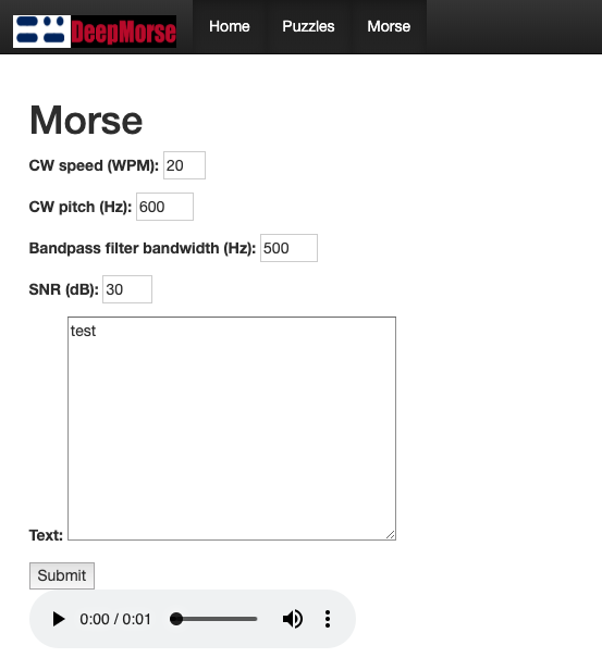


